Discovery of sparse, reliable omic biomarkers with Stabl

Abstract

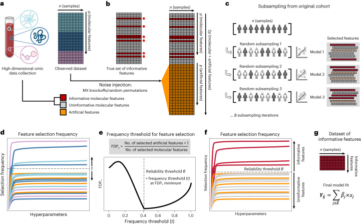
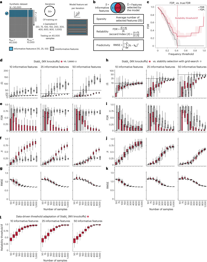
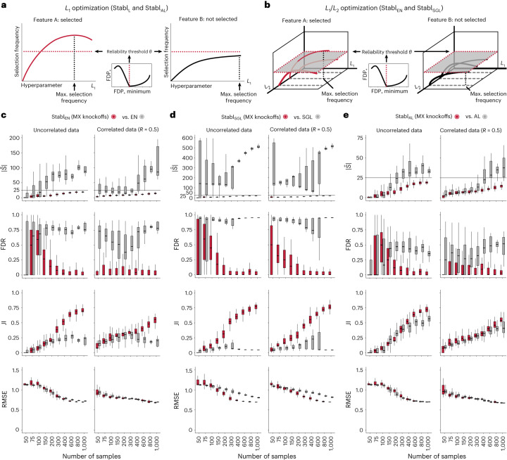
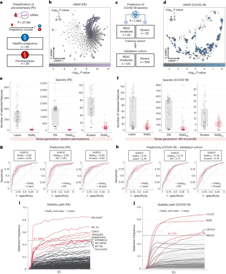
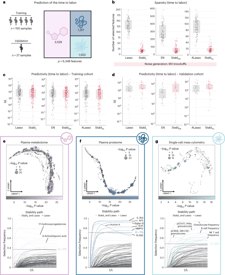
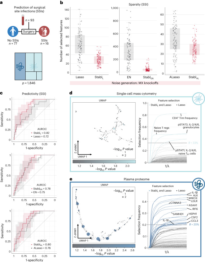
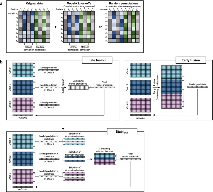
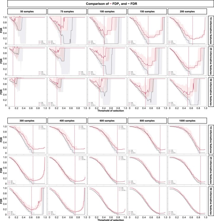
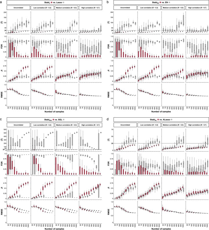
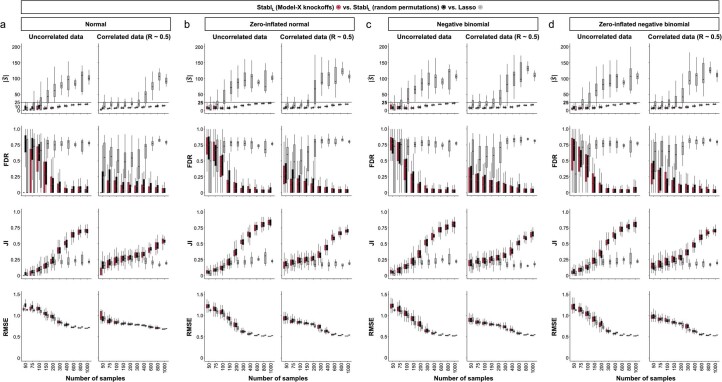
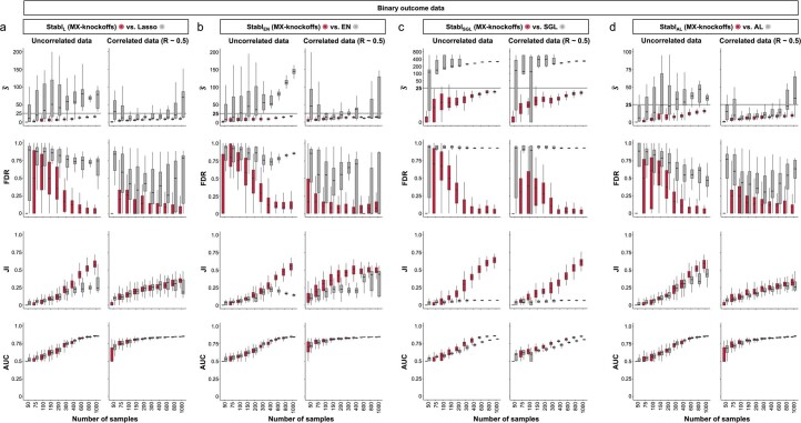
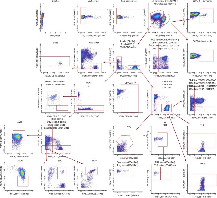
Adoption of high-content omic technologies in clinical studies, coupled with computational methods, has yielded an abundance of candidate biomarkers. However, translating such findings into bona fide clinical biomarkers remains challenging. To facilitate this process, we introduce Stabl, a general machine learning method that identifies a sparse, reliable set of biomarkers by integrating noise injection and a data-driven signal-to-noise threshold into multivariable predictive modeling. Evaluation of Stabl on synthetic datasets and five independent clinical studies demonstrates improved biomarker sparsity and reliability compared to commonly used sparsity-promoting regularization methods while maintaining predictive performance; it distills datasets containing 1,400-35,000 features down to 4-34 candidate biomarkers. Stabl extends to multi-omic integration tasks, enabling biological interpretation of complex predictive models, as it hones in on a shortlist of proteomic, metabolomic and cytometric events predicting labor onset, microbial biomarkers of pre-term birth and a pre-operative immune signature of post-surgical infections. Stabl is available at https://github.com/gregbellan/Stabl .

Fig. 1. Overview of the Stabl algorithm.

a, An original dataset of size n × p is obtained from measurement of p molecular features in each of n samples. b, Among the observed features, some are informative (related to the outcome, red), and others are uninformative (unrelated to the outcome, gray). p artificial features (orange), all uninformative by construction, are injected into the original dataset to obtain a new dataset of size n × 2p. Artificial features are constructed using MX knockoffs or random permutations. c, B subsample iterations are performed from the original cohort of size n. At each iteration k, SRM models varying in their regularization parameter(s) λ are fitted on the subsample, resulting in a different set of selected features for each iteration. d, For a given λ, B sets of selected features are generated in total. The proportion of sets in which feature i is present defines the feature selection frequency f_i(λ). Plotting f_i(λ) against 1/λ yields a stability path graph. Features whose maximum frequency is above a frequency threshold (t) are selected in the final model. e, Stabl uses the reliability threshold (θ), obtained by computing the minimum value of the FDP₊ (Methods). f,g, The feature set with a selection frequency larger than θ (that is, reliable features) is included in a final predictive model.

Fig. 2. Synthetic dataset benchmarking against Lasso.

a, A synthetic dataset consisting of n = 50,000 samples × p = 1,000 normally distributed features was generated. Some features are correlated with the outcome (informative features, light blue), whereas the others are not (uninformative features, gray). Forty thousand samples are held out for validation. Out of the remaining 10,000, 50 sets of sample sizes n ranging from 50 to 1,000 are drawn randomly to assess model performance. The Stabl_SRM framework is used using Lasso (Stabl_L) with MX knockoffs for noise generation. Performances are tested on continuous outcomes (regression tasks). b, Sparsity (average number of selected features, $\mid \widehat{S}\mid$), reliability (true FDR and JI) and predictivity (RMSE) metrics used for performance evaluation. c, The FDP₊ (red line; 95% CI, red shading) and the true FDR (gray line; 95% CI, gray shading) as a function of the frequency threshold (example shown for n = 150 samples and 25 informative features; see Extended Data Fig. 3 for other conditions). The FDP₊ estimate approaches the true FDR around the reliability threshold, θ. d–g, Sparsity (d), reliability (FDR, e; JI, f) and predictivity (RMSE, g) performances of Stabl_L (red box plots) and Lasso (gray box plots) with increasing number of samples (n, x axis) for 10 (left panels), 25 (middle panels) or 50 (right panels) informative features. h–k, Sparsity (h), reliability (i and j) and predictivity (k) performances of models built using a data-driven reliability threshold θ (Stabl_L, red box plots) or grid search-coupled SS (gray box plots). l, The reliability threshold chosen by Stabl_L shown as a function of the sample size (n, x axis) for 10 (left panel), 25 (middle panel) or 50 (right panel) informative features. Boxes indicate median and IQR; whiskers indicate 1.5× IQR.

Fig. 3. Extension of the Stabl_SRM framework to EN, SGL and AL: synthetic dataset benchmarking.

The Stabl_SRM framework is benchmarked against various SRMs, including EN (Stabl_EN), SGL (Stabl_SGL) and AL (Stabl_AL), respectively. a,b, Diagrams depict the strategy for identifying the maximum selection frequency for each feature across one (L₁ for Lasso and AL, a) or two (L₁/L₂ for EN and SGL, b) regularization parameters before minimizing the FDP₊. c–e, Sparsity ($\mid \widehat{S}\mid$), reliability (FDR and JI) and predictivity (RMSE) performances of Stabl_SRM (red box plots) are compared to their respective SRM (gray box plots) in n = 50 independent experiments for each number of samples for Stabl_EN (c), Stabl_SGL (d) and Stabl_AL (e). Synthetic modeling experiments performed on normally distributed datasets containing S = 25 informative features with uncorrelated (left panels) or intermediate correlation structures (right panels) are shown. For all correlated datasets, the target correlation between informative features is set at a Pearson correlation coefficient, R, of 0.5, yielding a covariance matrix with approximately the target correlation (R ≈ 0.5). Results with low or high correlation structures are shown in Extended Data Fig. 7. Performances are shown for regression tasks. Results for classification tasks are shown in Supplementary Table 10. Box plots indicate median and IQR; whiskers indicate 1.5× IQR.

Fig. 4. Stabl’s performance on transcriptomic and proteomic data.

a, Clinical case study 1: classification of individuals with normotensive pregnancy or PE from the analysis of circulating cfRNA sequencing data. The number of samples (n) and features (p) are indicated. b, UMAP visualization of the cfRNA transcriptomic features; node size and color are proportional to the strength of the association with the outcome. c, Clinical case study 2: classification of mild versus severe COVID-19 in two independent patient cohorts from the analysis of plasma proteomic data (Olink). d, UMAP visualization of the proteomic data. Node characteristics as in b. e,f, Sparsity performances (the number of features selected across n = 100 CV iterations, median and IQR) on the PE (e) and COVID-19 (f) datasets for Stabl_L (left), Stabl_EN (middle) and Stabl_AL (right). g,h, Predictivity performances (AUROC, median and IQR) on the PE (g) and COVID-19 (h, validation set; training set shown in Supplementary Table 5) datasets for Stabl_L (left), Stabl_EN (middle) and Stabl_AL (right). Stabl_SRM performances are shown using random permutations for the PE dataset and MX knockoffs for the COVID-19 dataset. Median and IQR values comparing Stabl_SGL performances to the cognate SRM are listed numerically in Supplementary Table 5. Results in the COVID-19 dataset using random permutations are also shown for Stabl_L in Supplementary Table 5. i,j, Stabl_L stability path graphs depicting the relationship between the regularization parameter and the selection frequency for the PE (i) and COVID-19 (j) datasets. The reliability threshold (θ) is indicated (dotted line). Features selected by Stabl_L (red lines) or Lasso (black lines) are shown. Significance between outcome groups was calculated using a two-sided Mann–Whitney test. Box plots indicate median and IQR; whiskers indicate 1.5× IQR.

Fig. 5. Stabl’s performance on a triple-omic data integration task.

a, Clinical case study 3: prediction of the time to labor from longitudinal assessment of plasma proteomic (SomaLogic), metabolomic (untargeted mass spectrometry) and single-cell mass cytometry data in two independent cohorts of pregnant individuals. b, Sparsity performances (number of features selected across CV iterations, median and IQR) for Stabl_L (left), Stabl_EN (middle) and Stabl_AL (right) compared to their respective SRM (late-fusion data integration method) across n = 100 CV iterations. c,d, Predictivity performances as squared error (SE) on the training (n = 150 samples, c) and validation (n = 27 samples, d) datasets for Stabl_L (left), Stabl_EN (middle) and Stabl_AL (right). Stabl_SRM performances are shown using MX knockoffs. Results using random permutations are shown for Stabl_L in Supplementary Table 5. Median and IQR values comparing Stabl_SRM performances to their cognate SRMs are listed in Supplementary Table 5. e–g, UMAP visualization (upper) and stability path (lower) of the metabolomic (e), plasma proteomic (f) and single-cell mass cytometry (g) datasets. UMAP node size and color are proportional to the strength of association with the outcome. Stability path graphs denote features selected by Stabl_L. The data-driven reliability threshold θ is computed for each individual omic dataset and is indicated by a dotted line. Significance of the association with the outcome was calculated using Pearson’s correlation. Box plots indicate median and IQR; whiskers indicate 1.5× IQR.

Fig. 6. Candidate biomarker identification using Stabl for analysis of a newly generated multi-omic clinical dataset.

a, Clinical case study 5: prediction of post-operative SSIs from combined plasma proteomic and single-cell mass cytometry assessment of pre-operative blood samples in patients undergoing abdominal surgery. b, Sparsity performances (the number of features selected across n = 100 CV iterations) for Stabl_L (left), Stabl_EN (middle) and Stabl_AL (right) compared to their respective SRMs (late-fusion data integration method). c, Predictivity performances (AUROC) for Stabl_L (upper), Stabl_EN (middle) and Stabl_AL (lower). Stabl_SRM performances are shown using MX knockoffs. Results using random permutations are shown in Supplementary Table 5. Median and IQR values comparing Stabl_SRM performances to their cognate SRMs are listed in Supplementary Table 5. d,e. UMAP visualization (left) and stability path (right) of the mass cytometry (d) and plasma proteomic (e) datasets. UMAP node size and color are proportional to the strength of association with the outcome. Stability path graphs denote features selected by Stabl_L. The data-driven reliability threshold θ is computed for individual omic datasets and indicated by a dotted line. Significance of the association with the outcome was calculated using a two-sided Mann–Whitney test. Box plots indicate median and IQR; whiskers indicate 1.5× IQR.

Extended Data Fig. 1. Infographics for noise injection methods and multi-omic data integration with StablSRM.

A. Noise injection methods. Left panel depicting the original dataset with n samples and p features with strong correlation between features f! and f" as well as medium correlation between f# and f$. Middle panel showing MX knockoffs as noise injection method where generated artificial features preserve the original features’ correlation structure. Right panel showing random permutations as alternative noise generation method, which does not preserve the correlation structure. B. Multi-omic data integration with StablSRM. Early fusion approaches of multi-omic data integration combine all features of all omics to a concatenated dataset to derive a multivariate model. Late fusion approaches build predictive models on each omic layer individually, then concatenate the model predictions together and build a predictive model. StablSRM’s method builds models in a bootstrapping fashion on each omic individually to select the informative features, then concatenates all selected (informative) features and builds a final predictive model on all selected features.

Extended Data Fig. 2. Comparison of FDP₊ and FDR in synthetic dataset benchmarking.

On the generated synthetic dataset, the FDP₊ and the true FDR were assessed for different dataset sizes ranging from n = 50 to 1000 samples with 10 (upper panels), 25 (middle panels), or 50 (lower panels) informative features. The FDP₊ (red line) and the true FDR (black line) are shown as a function of the frequency threshold. The selected reliability threshold (θ, red dotted line) varied across conditions. Boxes in box plots indicate the median and interquartile range (IQR), with whiskers indicating 1.5 × IQR.

Extended Data Fig. 3. Effect of varying numbers of artificial features on the computation of FDP₊.

On the generated synthetic dataset, the FDP₊ and the true FDR were assessed for a varying number of artificial features on a dataset of n = 200 samples and 10 (upper panels), 25 (middle panels), or 50 (lower panels) informative features within p = 1000 features. The FDP₊ (red line) and the true FDR (black line) are shown as a function of the frequency threshold. Increasing the number of artificial features allows for a more accurate estimation of the reliability threshold (θ, red dotted line). Boxes in box plots indicate the median and interquartile range (IQR), with whiskers indicating 1.5 × IQR.

Extended Data Fig. 4. Stabl_L’s performance on synthetic data with varying number of total features compared to Lasso.

Synthetic datasets differing in the number of features were generated as described in Fig. 2. Sparsity (∣Ŝ∣, a) reliability (FDR, b, and JI, c), and predictivity (RMSE, d) of Stabl_L (red box plots) and Lasso (grey box plots) as a function of the number of samples (n, x-axis) for 10 (left), 25 (middle), or 50 (right) informative features within p = 100, 500, 1000, 2500, 5000, 7500, and 10000 total number of features. Boxes in box plots indicate the median and interquartile range (IQR), with whiskers indicating 1.5 × IQR.

Extended Data Fig. 5. Reliability performance of selection frequency (Stabl_L) and beta coefficients (Lasso) to distinguish true positive and true negative features.

Beta coefficients assigned by Lasso and feature selection frequency assigned by Stabl were used to distinguish true positive and true negative features in a synthetic dataset with p = 1000 total features. The AUROC for this procedure is shown as a function of the number of samples (n, x-axis) for 10 (left panels), 25 (middle panels), or 50 (right panels) informative features. Boxes in box plots indicate the median and interquartile range (IQR), with whiskers indicating 1.5 × IQR.

Extended Data Fig. 6. Stabl_L’s performance on synthetic data with varying number of total features compared to SS with fixed frequency thresholds.

Synthetic datasets differing in the number of total features were generated as described in Fig. 2. Sparsity (∣Ŝ∣, a), reliability (FDR, b, and JI, c), and predictivity (RMSE, d) of Stabl_L (red lines) and stability selection with fixed frequency threshold of 30% (light grey lines), 50% (dark grey lines), or 80% (black lines) as a function of the number of samples (n, x-axis) for 10 (left), 25 (middle), or 50 (right) informative features within p = 100, 500, 1000, 2500, 5000, 7500, and 10000 total number of features. Boxes in box plots indicate the median and interquartile range (IQR), with whiskers indicating 1.5 × IQR.

Extended Data Fig. 7. Stabl’s performance on synthetic data with different correlation structures.

Synthetic datasets differing in correlation structure (low, medium, or high) were generated as described in Fig. 3. Sparsity (∣Ŝ∣, upper panels), reliability (FDR and JI, middle panels), and predictivity performances (AUROC, lower panels) for Stabl_L (a), Stabl_EN (b), Stabl_SGL (c), and Stabl_AL (d) (red box plots) and Lasso (grey box plots) as a function of the number of samples (n, x-axis) for 10 (left panels), 25 (middle panels), or 50 (right panels) informative features. Boxes in box plots indicate the median and interquartile range (IQR), with whiskers indicating 1.5 × IQR.

Extended Data Fig. 8. Stabl_L’s performance with MX knockoffs or random permutations on synthetic data with normal and non-normal distributions compared to Lasso.

Synthetic datasets differing in distribution were generated using the Normal to Anything (NORTA) framework, as described in methods. Sparsity (∣Ŝ∣, upper panels), reliability (FDR and JI, middle panels), and predictivity performances (RMSE, lower panels) of Stabl_L (MX knockoffs, red box plots, or random permutations, black box plots), and Lasso (grey box plots) as a function of the number of samples (n, x-axis) for synthetic data with a normal distribution (a), zero-inflated normal distribution (b), negative binomial distribution (c), or zero-inflated negative binomial distribution (d). The results are shown for datasets with 25 informative features in the context of uncorrelated (left panels) or correlated (right panels, intermediate correlation, R ~ 0.5) data for regression tasks (continuous outcomes). Results obtained for other scenarios, including other SRMs (EN, SGL, and AL), correlation structures (low, R ~ 0.2, high, R ~ 0.7), and classification tasks are listed in Table S2. Boxes in box plots indicate the median and interquartile range (IQR), with whiskers indicating 1.5 × IQR.

Extended Data Fig. 9. Stabl’s performance on synthetic data with binary outcomes.

Synthetic datasets with binary outcome variables were generated as described in Fig. 3. Sparsity (∣Ŝ∣), reliability (FDR and JI), and predictivity (RMSE) performances of StablSRM (red box plots) compared to the respective SRM (grey box plots) as a function of the sample size (n, x-axis) for Stabl_L (a), Stabl_EN (b), Stabl_SGL (c), and Stabl_AL (d). Scenarios with 25 informative features and uncorrelated (left panels) or intermediate feature correlation structures (Spearman R ~ 0.5, right panels) are shown. Boxes in box plots indicate the median and interquartile range (IQR), with whiskers indicating 1.5 × IQR.

Extended Data Fig. 10. Gating strategy for mass cytometry analyses (SSI dataset).

Live, non-erythroid cell populations were used for analysis.

References

1. Subramanian, I., Verma, S., Kumar, S., Jere, A. & Anamika, K. Multi-omics data integration, interpretation, and its application. Bioinform. Biol. Insights14, 1177932219899051 (2020). - PMC - PubMed
1. Wafi, A. & Mirnezami, R. Translational -omics: future potential and current challenges in precision medicine. Methods151, 3–11 (2018). - PubMed
1. Jackson, H. W. et al. The single-cell pathology landscape of breast cancer. Nature578, 615–620 (2020). - PubMed
1. Fourati, S. et al. Pan-vaccine analysis reveals innate immune endotypes predictive of antibody responses to vaccination. Nat. Immunol.23, 1777–1787 (2022). - PMC - PubMed
1. Dunkler, D., Sánchez-Cabo, F. & Heinze, G. Statistical analysis principles for omics data. Methods Mol. Biol.719, 113–131 (2011). - PubMed