Multifractality in spin glasses

Abstract

We unveil the multifractal behavior of Ising spin glasses in their low-temperature phase. Using the Janus II custom-built supercomputer, the spin-glass correlation function is studied locally. Dramatic fluctuations are found when pairs of sites at the same distance are compared. The scaling of these fluctuations, as the spin-glass coherence length grows with time, is characterized through the computation of the singularity spectrum and its corresponding Legendre transform. A comparatively small number of site pairs controls the average correlation that governs the response to a magnetic field. We explain how this scenario of dramatic fluctuations (at length scales smaller than the coherence length) can be reconciled with the smooth, self-averaging behavior that has long been considered to describe spin-glass dynamics.

Keywords: disorder systems; fractal dimensions; intermittency; large scale simulations.

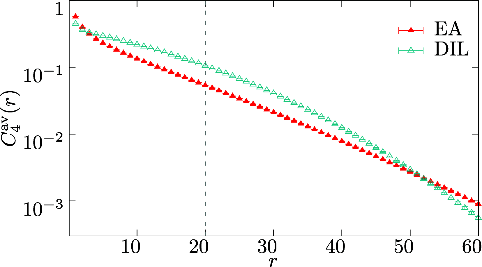
Fig. 1.

The correlation function, Eq. 10, as computed for the three-dimensional Ising diluted ferromagnet (DIL) and for the Ising spin glass (EA), versus distance $r$. Data were obtained in systems of linear size $L=160$ with coherence length $\xi (t_{\mathrm{w}})=20$ (dashed vertical line) at temperature $T=0.9$—recall that $T_{\mathrm{c}}\approx 1.1$ for EA (32). As explained in Methods, the coherence length is computed from the integral $I_2={\int }_0^{\infty }{r}^2{C}_4^{\text{av}}(r)\mathrm{d}r$ (the integrand is shown in the SI Appendix).

Fig. 2.

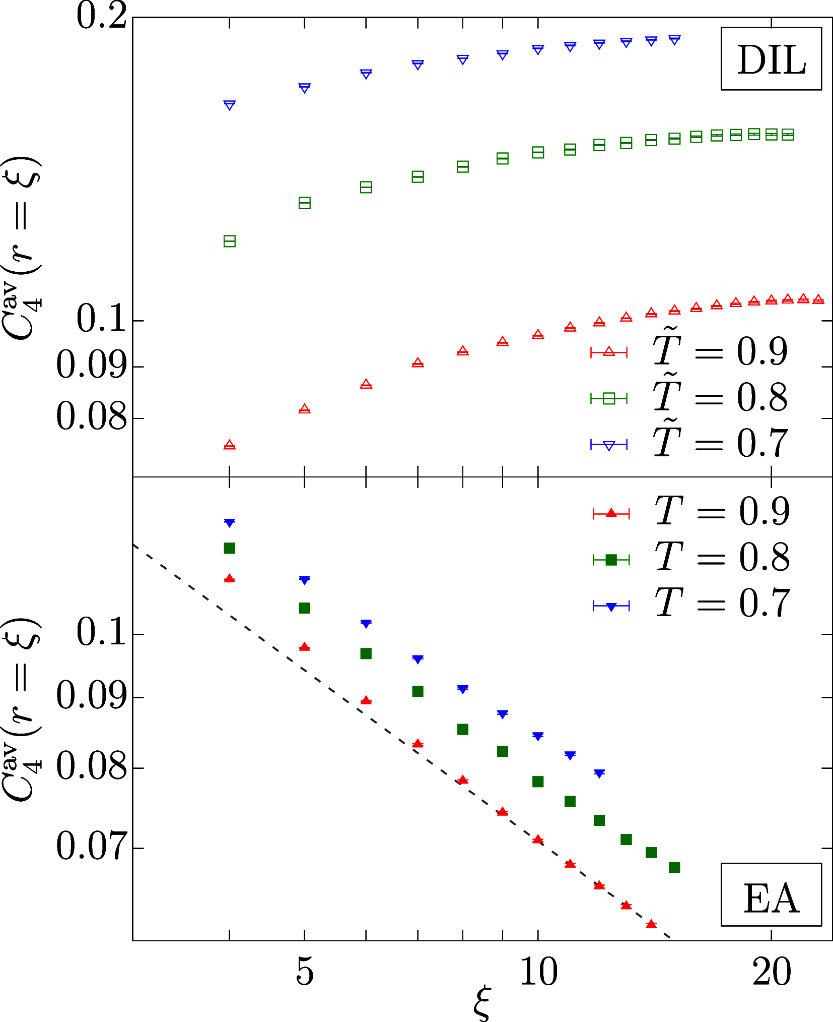
Correlation function $C_4^{\text{av}}(r=\xi (t_{\mathrm{w}}))$, see Eq. 10 versus the coherence length $\xi (t_{\mathrm{w}})$, as computed for DIL (Top) and for EA (Bottom) at temperatures $T,\tilde{T}=0.9,0.8$ and $0.7$ (see Methods for a complete definition of $\tilde{T}$). Error bars are smaller than the point size. The dashed line is our fit to Eq. 2, with $q=1$, for EA at $T=0.9$ (to avoid scaling corrections, we fit in the range $\xi (t_{\mathrm{w}})\in [10,20]$, see SI Appendix for further information). Note that, while the DIL $C_4^{\text{av}}(r=\xi (t_{\mathrm{w}}))$ tends to a $T$-dependent positive limit for large coherence length (which excludes multiscaling at $T<T_{\text{c}}$), the spin-glass correlation functions steadily decrease with $\xi (t_{\mathrm{w}})$.

Fig. 3.

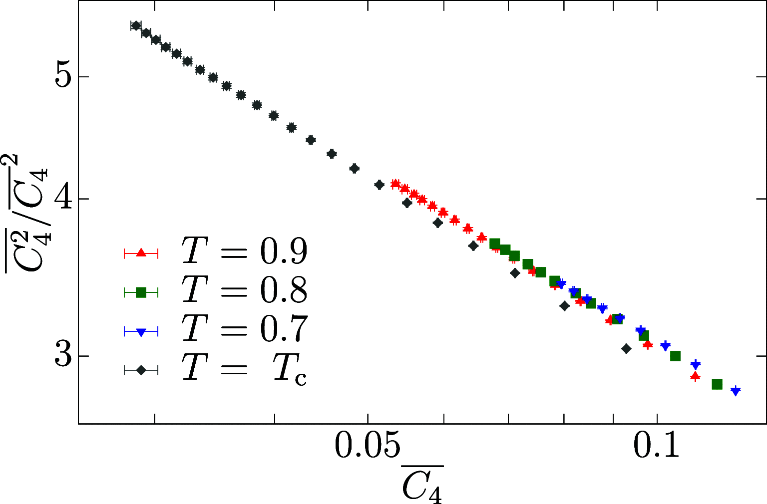
Ratio of the second moment of the spin-glass correlation function $C_4$ computed at $r=\xi (t_{\mathrm{w}})$, $\overline{C_4^2}$, to the squared first moment, ${\overline{C_4}}^2$, as a function of $\overline{C_4}$. We show the data for all temperatures considered in this work. $\overline{C_4}$ tends to zero as the coherence length $\xi (t_{\mathrm{w}})$ gets large, recall Fig. 2. Note that $\overline{C_4^2}/{\overline{C_4}}^2$ scales with $\overline{C_4}$ as a power law, which indicates that in the scaling limit (i.e., $\xi (t_{\mathrm{w}})\to \infty$ or $\overline{C_4}\to 0$) the order of magnitude of $\overline{C_4^2}$ is larger than the one of ${\overline{C_4}}^2$. Data in the glassy phase, $T<T_{\mathrm{c}}$, roughly follow the same scaling curve. At the critical point, there is still a power type relation with a slightly different exponent. Error bars are smaller than the points size. The same data are shown as a function of $\xi (t_{\mathrm{w}})$ in SI Appendix.

Fig. 4.

Grayscale representation of the order-of-magnitude modulating factor $M(\mathit{x},\mathit{r},t_{\mathrm{w}})$, see Eq. 1, computed for site $\mathit{x}=(64,64,64)$ of a sample with coherence length $\xi (t_{\mathrm{w}})=20$, at $T=0.9$, with an $N_{\mathrm{R}}=512$ estimator (Methods). We show results for displacement vectors $\mathit{r}=(r_x,r_y,r_z)$ in a cube $-40\le r_x,r_y,r_z\le 40$. The Top-Left panel depicts the three visible faces of the cube, while the other three panels show sections at $r_z=-20,0,20$, respectively. Our color code is darker the smaller $M(\mathit{x},\mathit{r},t_{\mathrm{w}})$ (hence, the more slowly correlations decay with distance). For ease of representation, we have chosen a color code linear between the minimal value of $M(\mathit{x},\mathit{r},t_{\mathrm{w}})$ and 2.5. Displacements $\mathit{r}$ with $M(\mathit{x},\mathit{r},t_{\mathrm{w}})>2.5$ are depicted as if $M(\mathit{x},\mathit{r},t_{\mathrm{w}})=2.5$. See SI Appendix for more examples of this modulating factor.

Fig. 5.

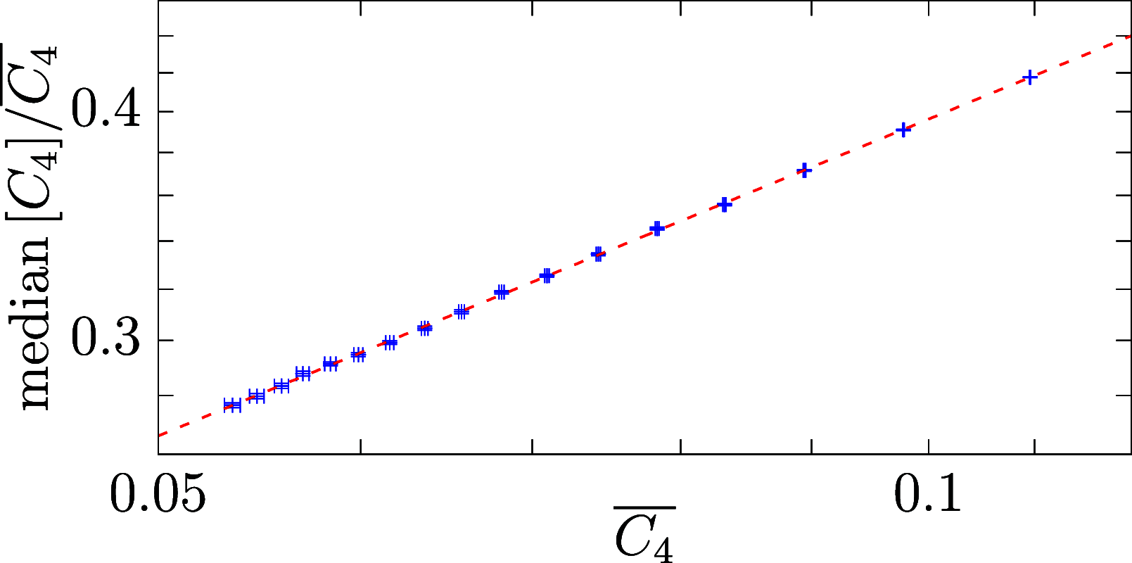
Median of the distribution $P[C_4(r=\xi )]$ in units of the first moment, $\overline{C_4}(r=\xi )$, versus $\overline{C_4}(r=\xi )$, as computed for the spin glass at temperature $T=0.9$. We show data in the logarithmic scale. Therefore, the dashed line (a power-law fit with exponent $\sim 0.5$, see SI Appendix for details) appears as a straight line.

Fig. 6.

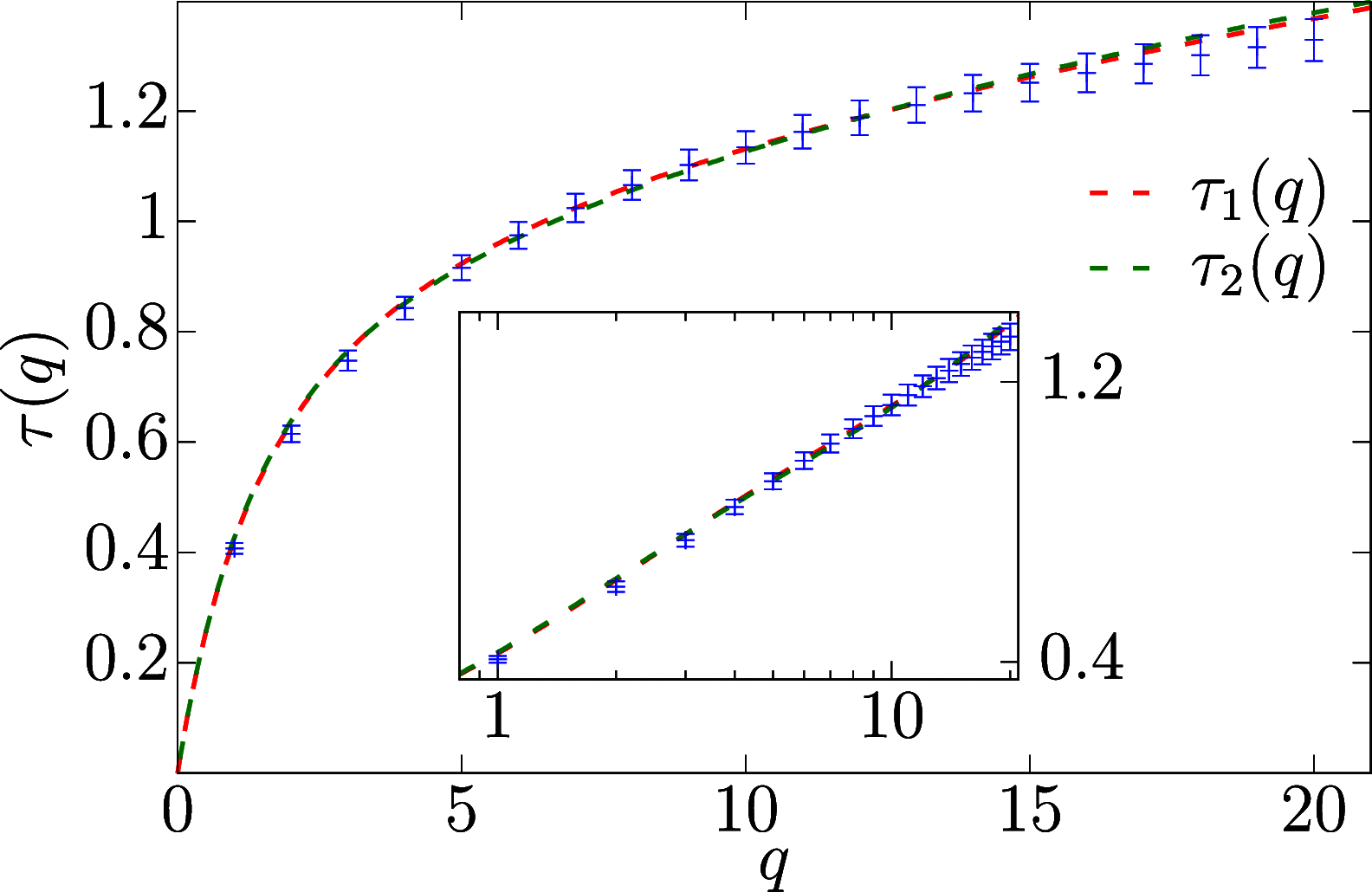
Scaling exponent $\tau (q)$ for the $q$-th moment $\overline{C_4{(r=\xi )}^q}\sim {\xi }^{-\tau (q)}$ computed from simulations of the Ising spin glass at $T=0.9$ (see SI Appendix for results at $T_{\mathrm{c}}$). The nonlinear behavior is a strong indication of multifractality. The dashed lines are fits to the functional forms in Eq. 3 (the goodness-of-fit statistics are presented in the SI Appendix). The inset presents the same data as a function of $log(q)$.

Fig. 7.

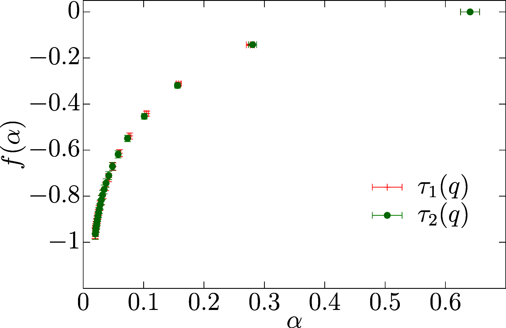
Legendre transformation $f(\alpha )$ of function $\tau (q)$, see Eq. 7, as a function $\alpha =\mathrm{d}\tau /\mathrm{d}q$, computed from the fitting ansätze in Eq. 3. Errors on both axes have been obtained as explained in Methods (for further details, see ref. 50). Since $f(\alpha )$ is the large-deviations function of the decay rate $C_4(r=\xi )\sim r^{-\alpha }$, the data show that the majority of sites have the median decay rate of approximately $0.65$, much larger than the mean decay rate $\alpha \approx 0.4$.

References

1. U. Frisch, G. Parisi, “On the singularity structure of fully developed turbulence” in Turbulence and Predictability in Geophysical Fluid Dynamics and Climate Dynamics (1983 International School of Physics "Enrico Fermi", Varenna), M. Ghil, R. Benzi, G. Parisi, Eds. (North-Holland, Amsterdam, 1985).
1. Harte D., Multifractals. Theory and Applications (Chapman and Hall/CRC, New York, NY, ed. 1, 2001).
1. Wilson K. G., Problems in Physics with many Scales of Length. Sci. Am. 241, 158–179 (1979).
1. Parisi G., Statistical Field Theory (Addison-Wesley, 1988).
1. Barnsley M., Fractals Everywhere (Dover Publications, Inc., Mineola, NY, ed. 3, 2012).
LinkOut - more resources