A compendium of genetic regulatory effects across pig tissues

Abstract

The Farm Animal Genotype-Tissue Expression (FarmGTEx) project has been established to develop a public resource of genetic regulatory variants in livestock, which is essential for linking genetic polymorphisms to variation in phenotypes, helping fundamental biological discovery and exploitation in animal breeding and human biomedicine. Here we show results from the pilot phase of PigGTEx by processing 5,457 RNA-sequencing and 1,602 whole-genome sequencing samples passing quality control from pigs. We build a pig genotype imputation panel and associate millions of genetic variants with five types of transcriptomic phenotypes in 34 tissues. We evaluate tissue specificity of regulatory effects and elucidate molecular mechanisms of their action using multi-omics data. Leveraging this resource, we decipher regulatory mechanisms underlying 207 pig complex phenotypes and demonstrate the similarity of pigs to humans in gene expression and the genetic regulation behind complex phenotypes, supporting the importance of pigs as a human biomedical model.

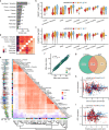
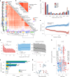
Fig. 1. Characteristics of samples in the pilot phase of PigGTEx project.

a, Clustering of 7,095 RNA-seq samples based on the normalized expression (log₁₀-transformed TPM) of 6,500 highly variable genes, defined as the top 20% of genes with the largest s.d. of TPM across samples. b, The same sample clustering as a but based on normalized alternative splicing values (PSI) of 6,500 highly variable spliced introns, defined as the top 13% of spliced introns with the largest s.d. of PSI across samples. c, Principal component analysis of samples based on 12,207 LD-independent (r² < 0.2) SNPs. The left panel is for whole-genome sequencing samples (n = 1,602) in the PGRP, while the right one is for RNA-seq samples (n = 7,008) with successful genotype imputations. d, Sample sizes of 34 tissues, cell types and organ systems (all referred to as ‘tissues’) used for molQTLs mapping. e, Clustering of 34 tissues based on the median expression of all 31,871 Ensembl annotated genes (v100) across samples within tissues, representing embryo, endodermal, mesodermal and ectodermal lineages.

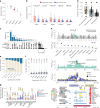
Fig. 2. molQTL discovery.

a, Pearson’s r between the proportion of detectable eGenes and sample size across 34 tissues. b, Proportions of detectable eMolecule (blue) and specific molQTL (red) for different molecular phenotypes in 34 tissues. * indicates the interaction of cis-eQTLs (ieQTL). Cell type* and Ancestry* are for cell-type ieQTL (cieQTL) and breed/ancestry ieQTLs (bieQTL), respectively. c, Distribution and the average number of independent cis-eQTL per gene. Tissues (x axis) are ordered by increasing sample size. The color key is the same as in a. d, Number of eGenes (triangle) and average number of independent cis-eQTL (square). e, The comparison of cis-h² (blue) and median expression levels (red) of genes with different numbers of detectable independent cis-eQTL across tissues. The top labels show nominal P values (uncorrected for multiple testing) from one-sided Student’s t tests. f, Internal validation of cis-eQTL. Bars represent Pearson’s r of the normalized effects of cis-eQTL between validation and discovery groups. Points represent the π₁ statistic measuring the replication rate of cis-eQTL. g, Spearman’s ρ of effect sizes (aFC in log₂ scale) between cis-eQTL and ASE at matched loci (n = 4,417) in muscle. h, A cis-eQTL (rs331530041) of EMG1 in muscle is shared across eight ancestry groups. i, Spearman’s correlation of the cis-eQTL effects between eight breeds of the muscle (left) and between muscle and other 33 tissues (right). The P value is obtained from a two-sided Wilcoxon rank-sum test. j, Proportion of bieQTL that are validated with the ASE approach. The number of validated bieQTLs out of the total number of bieQTLs tested is shown to the right of each bar. k, Effect of eVariant (rs344529295) of GRHPR interacted with the Duroc ancestry enrichment in muscle. The two-sided P value is calculated by the linear regression bieQTL model. The lines are fitted by a linear regression model using the geom_smooth function from ggplot2 (v3.3.2) in R (v4.0.2). l, Proportion of cieQTL that are validated by the ASE approach. m, Effect of eVariant (rs344431919) of FGD2 interacted with monocyte enrichment in blood. The two-sided P value is calculated by the linear regression cieQTL model. The lines are fitted using the same method as in k. aFC, allelic fold change.

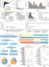
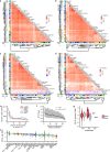
Fig. 3. Tissue-sharing pattern of regulatory effects.

a, Heatmap of tissues depicting the corresponding pairwise Spearman’s correlation (ρ) of cis-eQTL effect sizes. Tissues are grouped by hierarchical clustering (bottom). Violin plots (left) represent Spearman’s ρ between the target tissue and other tissues. b, Similarity (measured by the median pairwise Rand index) of tissue-clustering patterns across ten data types. c, The overall tissue-sharing pattern of five molQTL types at LFSR < 5% obtained by MashR (v0.2-6). d, Relationships between the magnitude of tissue-sharing of cis-eQTL and their effect sizes (aFC, left), MAFs (middle) and distances to the TSS (right). The P values are obtained by Pearson’s correlation (r) test. The line and shading indicate the median and interquartile range, respectively. e, Conservation of DNA sequence (measured by the PhastCons score of 100 vertebrate genomes) of eGenes and non-eGenes regarding tissue-sharing. The line and shading indicate the mean and standard error, respectively. f, Counts of four types of SNP–gene pairs across 34 tissues. Ind., independent cis-eQTL; top., top cis-eQTL; multi., eGenes have identical or high LD (r² > 0.8) cis-eQTL in any two tissues; opp-multi., eGenes have an opposite direction of cis-eQTL effect between any two tissues. g, Scatter plots of cis-eQTL effect sizes of 48 common multi-eGenes in blood and testis. cis-eQTL with the same directional effect are colored blue (n = 36), and those with the opposite direction are colored red (n = 12). h, The cis-eQTL effects of ODF2L on chromosome 4 in blood and testis. Diamond symbols represent the top cis-eQTL of ODF2L. The two-sided P value is calculated by the linear regression cis-eQTL model.

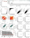
Fig. 4. Functional characterization of regulatory variants.

a,b, Fold enrichment (mean ± s.d.) for fine-mapped molQTLs in sequence ontologies (a) and 14 chromatin states (b). c, Enrichment of cis-eQTL in five types of enhancers. Each box includes enrichment of cis-eQTL from 34 tissues across enhancers. Blue dots represent enrichments from matching tissues. d, Enrichment of top three independent cis-eQTL in two chromatin states. TssA is for active TSS, while EnhA is for active enhancers. The P values are obtained by the two-sided Student t test. *P < 0.05 and NS indicates not significant. e, Enrichment (mean ± s.d.) of cis-eQTL within the same topologically associating domain of TSS of target genes. TADs are obtained from Hi-C data of five tissues. The cis-eQTL are grouped according to their distance to TSS. – and + means upstream and downstream, respectively. f, The landscape of BUD23 at multiple genomic features in muscle. The top plot shows that BUD23 and its second independent eVariant (rs790620973) are located within a TAD (the black triangle). The bottom is the Manhattan plot showing cis-eQTL results of BUD23. The violin plot shows the expression levels (log₁₀-transformed TPM) of BUD23 across three genotypes (AA, n = 9; GA, n = 131; GG, n = 1,181) of this eVariant in muscle. The two-sided P value is obtained from the linear regression cis-eQTL model.

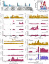
Fig. 5. Interpreting GWAS loci of complex traits using molQTL.

a, Enrichment (mean and 95% confidence interval) of GWAS variants with five types of molQTL in 34 tissues. b, Heritability of 16 complex traits of pig explained by independent molQTLs and those MAF-matched SNPs across 34 tissues. The top numerical labels are the nominal P values (uncorrected for multiple testing) based on the two-sided paired Student’s t test. c, Number of GWAS loci linked to eGenes through fastEnloc, SMR, S-PrediXcan and S-MultiXcan. The bottom point-line combinations of the upset plot represent the intersections of GWAS loci linked to eGenes by different methods. d, Proportion of three types of GWAS loci regarding the colocalization results, where 105 GWAS traits are shown in each category. No colocalization, GWAS loci that are not colocalized with any eGenes in 34 tissues. Not nearest gene, GWAS loci whose colocalized eGenes are not nearest genes to GWAS lead SNPs. Nearest gene, GWAS loci whose colocalized eGenes are the nearest ones. Each dot represents a complex trait. e, Proportion of significant colocalizations of GWAS loci with cis-eQTL at various significance levels of GWAS. f, The number of colocalized GWAS loci per eGene across 105 traits above. eGenes are classified into seven groups regarding the tissue-sharing pattern. Diamond indicates the mean value. g, The number of colocalized genes adjusted for tissue sample size and eGene discovery ratio in 14 tissues across 18 GWAS traits (detailed abbreviations in Supplementary Table 18). Top tissues are labeled. h, The association of ABCD4 with the average BFT. The top Manhattan plot represents the TWAS results of BFT in the small intestine, followed by the TWAS results of ABCD4 for BFT in 12 tissues being tested. The two following Manhattan plots show the colocalization of BFT GWAS (top) and cis-eQTL (bottom) of ABCD4 on chromosome 7 (chr 7) in both the brain and small intestine. The blue and yellow triangles indicate the top variants of ABCD4 in the small intestine (rs3473180467) and brain (rs1110461203), respectively. These two variants are in high LD (r² = 0.71). The bottom panel is for chromatin states around ABCD4.

Fig. 6. Conservation of gene expression, cis-eQTL and complex trait genetics between pigs and humans.

a, Enrichment (Fisher’s exact test) of pig eGenes with human eGenes across 17 matching tissues. Red triangles: matching tissues. b, Pearson’s correlation of eQTL effect size in orthologous genes (n = 15,944) between pigs and humans. c, Expression levels, TAU values and tissue-sharing levels for four groups of orthologous genes across 17 tissues in pigs. Neither, 3,993 non-eGenes in both species; human-specific, 8,174 eGenes; pig-specific, 3,882 eGenes; shared, 10,574 eGenes in both species. Two-sided Wilcoxon rank-sum test, ***P < 0.001. Diamond, median; error bar, upper/lower quartiles. d, LOEUF in the four groups of orthologous genes in ten evenly spaced expression level bins. One-sided Wilcoxon rank-sum test, NS P > 0.05, *P < 0.05, **P < 0.01 and ***P < 0.001. The diamond and error bar are the same as in c. e, Significance (−log₁₀(P)) of Pearson’s r of orthologous gene effect size between pig (n = 268) and human (n = 136) traits derived from TWAS. Each bar represents a pig–human trait pair in the same tissue (n = 11) and the within-domain blocks of color correspond to different human traits. The number of tested genes for each of the pairs is shown in Supplementary Table 30. The text in the middle of the circle represents the significant examples of pig–human trait pairs in different thresholds. For each example, it includes human trait (top), pig trait (bottom) and TWAS tissue (left). P_{cutoff 1}: FDR < 10% across all tested combinations. P_{cutoff 2}: Bonferroni-corrected P < 5% within each trait–tissue pair of humans. f, Differences in the number of significant genes (FDR < 5%) from cross-species (pig and human) meta-TWAS, compared to those from human TWAS. Supplementary Tables 18 and 29 present a detailed description of pig traits and human traits, respectively. g, FDR of discovered genes in human TWAS (RawTWAS) and cross-species meta-TWAS in the brain for BFT (pig) and weight (human). h, Pearson’s r between TWAS significances (color bar) of genes in pig BFT and their heritability enrichments (mean ± s.e.) in human weight. The orthologous genes were divided into ten evenly spaced bins by sorting the P values of TWAS in the brain of pig BFT. Shading: standard error of the fitting line.

Extended Data Fig. 1. Genotype calling and imputation and breed prediction.

a, Pearson’s correlation (r) between number of clean reads and number of called SNPs across 7,095 RNA-Seq samples. The P-value is obtained by Pearson’s r test. b, Distribution of the number of SNPs called from 7,095 RNA-Seq samples. c, Number of imputed SNPs (left, gray bars) from 7,008 RNA-Seq samples across 18 pig chromosomes after quality control (DR² ≥ 0.85, minor allele frequency ≥ 0.05). The red point represents the number of genes (right) in each chromosome in the Sscrofa11.1. assembly (Ensembl v100). d, Distribution of 42,523,218 SNPs from the Pig Genomics Reference Panel (PGRP) and 3,087,268 imputed SNPs used for molecular QTL (molQTL) mapping across eight genomic features. e, Minor allele frequency (MAF) of imputed SNPs in 7,008 RNA-Seq samples. f, Distribution of the number of imputed SNPs around 1 Mb of transcript start site (TSS) of 18,911 protein-coding genes. g, Concordance rate (CR) and squared correlation (r²) of imputed and observed genotypes in 50 evenly spaced MAF bins based on individuals that are not present in the PGRP. ‘ALL’ represents the entire variants. h, CR and r² of imputed genotypes from RNA-Seq only and those directly called from whole-genome sequence (WGS) data (red), and imputed genotypes (blue) from SNP array, respectively, in the same individuals. Point and whisker are mean and standard deviation, respectively. Labels of x-axis are breeds and number of individuals. i, CR and r² (median and interquartile) of imputed and observed genotypes in different genomic features. Point and whisker are median and interquartile, respectively. j, The overall pipeline utilized to predict missing breed labels for RNA-Seq samples. k, Estimated ancestry proportion of Duroc (n = 485), Landrace (n = 280), Yorkshire (n = 145), Landrace×Yorkshire (n = 165) and Duroc×Landrace×Yorkshire (n = 40) samples. l, Distribution of sample size of training and prediction sets in pure and cross breeds. m,n, Accuracy of breed prediction for pure breeds (m) and cross breeds (n) measured by cross-validation. The red triangle represents the sample size of the target breed.

Extended Data Fig. 2. Detection of duplicated individuals and confounders of RNA-Seq samples.

a, Distribution of identity-by-state (IBS) distances among 7,008 RNA-Seq samples, which are calculated using 12,207 LD-independent SNPs (r² < 0.2). b, Density of IBS distances that were computed using genotypes derived from RNA-Seq only and whole-genome sequence (WGS) or SNP array data in the same individuals (n = 227). c, Heatmap of IBS distance of 25 RNA-Seq samples from 9 individuals. The same color on the top of panel represents samples from the same individuals. True: true individual label; Assigned: assigned individual label using an IBS distance cutoff of 0.9. d, Pearson’s correlation (r) between IBS distance calculated from imputed genotypes and those calculated from WGS or SNP array data across four different populations. L×Y: Landrace and Yorkshire cross breed (n = 25); Duroc×DNXE: Duroc and Diannanxiaoer cross breed (n = 11); Duroc: Duroc pure breed (n = 37); D×L×Y: composite population with 1/4 Duroc, 1/2 Landrace and 1/4 Yorkshire (n = 179). e, Duplicated and remaining individuals in each of the 34 pig tissues used for molecular QTL mapping. Sample pairs with IBS > 0.9 were considered as duplicated individuals. f, Proportion of variance explained (PVE) by genotype principal components (PC) in each of 34 tissues (lines). g, Factor weight variance of probabilistic estimation of expression residual (PEER) factors in each of 34 tissues (lines). h, Proportion of variance (adjusted R²) of known confounders captured by the top 10 inferred PEER factors, calculated using the lm function in R (v4.0.2).

Extended Data Fig. 3. The pig gene expression atlas.

a, Tissue-specific expression of five transcript types reflected by the TAU score. PCG: protein-coding genes. b, Gene numbers (left), expression pattern (middle, transcripts per million, TPM), and enriched Gene Ontology (GO) terms (right) of tissue-specific genes in 34 tissues. c, Enrichment of muscle-specific genes in 15 chromatin states across 14 pig tissues. The red dots represent respective chromatin states in muscle. The blue line indicates enrichment fold = 1. d, Expression profiles of MYL2 gene across 34 tissues (left). The tissue color key is the same as in (b). Chromatin state distribution (right) around MYL2 in 14 pig tissues. In brief, red is for promoters, yellow for enhancers, blue for open chromatin and gray for repressed regions. e, Enrichment of tissue-specific genes for two active chromatin states across 11 tissues, which have both chromatin states and gene expression data. The dots represent enrichments from matching tissues. TssA is for active TSS (promoter), and EnhA for active enhancers. f, Comparison of genes with and without functional annotation (referred to as ‘annotated genes’ and ‘unannotated genes’, respectively) in gene co-expression modules at different biological layers. The gene co-repression analysis was conducted using five complementary methods, including WGCNA, ICA, PEER, MEGENA and CEMiTool. ‘All’ shows the combined results from the five methods. The functional annotation was based on the Gene Ontology database (version 2022-01-18). The plots from top to bottom include gene counts, expression level, PhastCons score from 100 vertebrate genomes, proportion of orthologous genes in humans and TAU values. Significant differences between annotated and unannotated genes were obtained using a two-sided Student t-test. ** means P < 0.01. g, An example of gene co-expression module in the pituitary, which includes 59 unannotated and 42 annotated genes, respectively. The functional annotated genes are significantly (P = 8 × 10⁻³) enriched in neuron apoptotic processes. The gray edges between genes represent Pearson’s correlations of expression across all 53 samples in the pituitary. h, The proportion of unannotated genes in each gene co-expression modules across 34 tissues.

Extended Data Fig. 4. Cis-heritability of gene expression across 34 pig tissues.

a, Distribution of estimated cis-heritability (cis-h²) of gene expression across 34 tissues. The black point represents the median of cis-h² of all tested genes in a tissue. b, Box plot showing the cis-h² estimates of genes across 34 tissues that are significant (likelihood ratio test P < 0.05) or non-significant, where 16,174 (93%) unique genes have significant cis-heritability in at least one tissue. The P value was calculated by two-sided Student t-test. c, The number of eGenes in each tested tissue, with 86% of the tested genes (red bar, left) are eGenes in at least one tissue. The blue points represent the number of tissue-specific eGenes.

Extended Data Fig. 5. Conditionally independent molecular QTLs (molQTL).

a, Distribution and average number (red dots, right y-axis) of conditionally independent cis-QTL per eMolecules across 34 tissues. Tissues (x-axis) are ordered by increasing sample size. b, Cumulative proportion of distance to the transcription start site (TSS) of target genes for conditionally independent cis-eQTL in each of 34 tissues. The meanings of the colors of curved lines are the same as the color key in panel (a). c,d, Comparison of distance to TSS (c) and effect size (|log₂(aFC)|) (d) among top three independent cis-eQTL per eGene across 34 tissues. The aFC is for allelic fold change. The P values were obtained by the two-sided Wilcoxon rank-sum test.

Extended Data Fig. 6. Validation of cis-eQTL.

a, Pearson’s correlation of combined summary statistics (for example, Z-score, slope and P-value (-log₁₀ scale)) of cis-eQTL for all the eGenes across 34 tissues between TensorQTL (linear model, LM) and fastGWA (mixed linear model, MLM). b, Pearson’s correlation of summary statistics for each eGene in each tissue between LM and MLM. c, Distribution of the Pearson’s correlations of Z-score between LM and MLM. d, Relationship between correlations of Z-score and the number of significant eQTL across all the eGenes. e, Correlation of P values derived from MLM and nominal (left) or permutation-corrected (right) P derived from LM for the lead eQTL of all the eGenes. f, Replication rates (π₁) of blood cis-eQTL between the PigGTEx discovery population (n = 386, Discovery) and the external datasets (n = 179). For π₁ calculation, rows are discovery populations, and columns are replication populations. The external datasets include whole-blood-cell RNA-Seq data and SNP Chip array (Chip) from 179 animals at two developmental stages (T1 and T2). The prefix ‘RNA’ and ‘Chip’ indicate imputed genotypes from RNA-Seq and SNP array, respectively. g, Spearman’s correlation (ρ) of effect size (z-scores) for blood cis-eQTL among the same populations above. h, Replication rates (π₁) of PigGTEx cis-eQTL in external validation datasets of three tissues, including muscle (n_PigGTEx = 1,321, n_external = 100), liver (n_PigGTEx = 501, n_external = 100) and duodenum (n_PigGTEx = 49, n_external = 100). The x-axis is the nominal P-value of cis-eQTL detected from dataset₂ and is significant in dataset₁ (that is, dataset₁ in dataset₂). i,j, Spearman’s correlation (ρ) of effect sizes (allelic fold change, aFC in log₂ scale) between cis-eQTL and matched allele-specific expression (ASE) loci in the liver (i) and brain (j). N indicates number of tested loci. The lines are fitted by a linear regression model using the geom_smooth function from ggplot2 (v3.3.2) in R (v4.0.2). The shading represents the standard error of the fitting line. k, Spearman’s correlation (ρ) of effect sizes between cis-eQTL and matched ASE loci across 34 tissues. Red dots indicate number of tested loci (right y-axis).

Extended Data Fig. 7. Breed sharing and interaction cis-eQTL (bieQTL).

a, Sample size of muscle RNA-Seq data across eight breed groups. b,c, Expression levels of NMNAT1 (b) and COMMD10 (c) at three genotypes of cis-eQTL in muscle across eight breed groups. d, The cis-eQTL discovered in each breed group (rows) that can be replicated (π₁) across all other breed groups (columns). e, The heatmap of tissues regarding the pairwise Spearman’s correlation (ρ) of cis-eQTL effect sizes. Tissues are grouped by hierarchical clustering (bottom). Violin plot (left) represents Spearman’s correlation between the target group and the rest. f, Pearson’s correlation (r) of effect size between cis-eQTL from the multi-breed meta-analysis (y-axis) and those from the combined muscle population (x-axis). The P value was obtained from Pearson’s r test. g, Overlap of cis-eQTL detected from the combined muscle population (Combined) and those detected in single-breed (Single) cis-eQTL mapping (shared in at least two breeds). h,i, Examples of bieQTL in muscle. Each dot in (h, CA14) and (i, ATE1) represents an individual and is colored by three genotypes. Gene expression levels and ancestry enrichment scores are inverse normal transformed. The two-sided P value is calculated by the linear regression bieQTL model. The lines are fitted by a linear regression model using the geom_smooth function from ggplot2 (v3.3.2) in R (v4.0.2).

Extended Data Fig. 8. Cell-type enrichment and interaction cis-eQTL (cieQTL).

a, Distribution of enrichment scores (percentage) of major cell types in samples of seven tested tissues (brain: n = 415, frontal cortex: n = 75, hypothalamus: n = 73, lung: n = 149, blood: n = 386, liver: n = 501, and spleen: n = 91). Each point and whisker indicate the mean value and standard deviation, respectively. b,c, Examples of cieQTL in blood. Each dot in (b, SCRN2) and (c, HIBADH) represents an individual and is colored by three genotypes. Gene expression levels and cell-type enrichment scores are inverse normal transformed. The two-sided P value was calculated by the linear regression cieQTL model. The lines are fitted by a linear regression model using the geom_smooth function from ggplot2 (v3.3.2) in R (v4.0.2). d–f, Pearson’s correlation (r) between allele-specific expression (ASE) effect sizes (allelic fold change, aFC) and specific cell-type enrichment scores for FGD2 with monocytes (d), SCRN2 with CD2⁻ γδ T cells (e) and HIBADH with CD4⁺ αβ T cells in the blood (f). The lines are fitted by a linear regression model using the geom_smooth function from ggplot2 (v3.3.2) in R (v4.0.2). The shading represents the standard error of the fitting line. g, ASE validation rate (π₁) of breed/cell-type interaction QTL (bieQTL and cieQTL) across tissues with ≥ 5 detectable bieQTL or cieQTL.

Extended Data Fig. 9. Tissue-sharing and specificity patterns of molecular QTL (molQTL).

a–d, The heatmap of tissues regarding the pairwise Spearman’s correlation (ρ) of molQTL effect sizes, that is, cis-sQTL (a), cis-eeQTL (b), cis-lncQTL (c) and cis-enQTL (d). Tissues are grouped by the hierarchical clustering (bottom). Violin plot (left) represents Spearman’s correlations between the target tissue and the rest. e, Distribution of number of tissues having METASOFT activity (m-value > 0.7) for each of molQTL. MolPhe: molecular phenotype. f, Pearson’s correlation (r) between number of tissues an eGene expressed in (transcript per million, TPM > 0.1) and its cis-eQTL effect sizes (|aFC(log₂)|). The aFC is for allelic fold change. The line and shading indicate the median and interquartile range, respectively. g, Expression levels (adjusted TMM) of ODF2L at three genotypes of top cis-eQTL (rs329043485) in blood and testis. TMM: trimmed mean of M-value normalized expression levels. There are 337, 47 and 2 samples for A/A, A/C and C/C genotypes in blood, respectively, and 148, 34 and 2 in testis, respectively. h, Expression levels (log₂TMM) of ODF2L across 34 tissues. Tissues are ordered (from smallest to largest) by the median expression values.

Extended Data Fig. 10. Complementarity of molecular QTL (molQTL) in interpreting GWAS loci.

a, Number of GWAS loci linked to cis-eQTL, cis-sQTL, cis-eeQTL, cis-lncQTL and cis-enQTL in 34 tissues based on four different integrative methods, including colocalization (fastEnloc), Mendelian randomization (SMR), single-tissue transcriptome-wide association studies (TWAS, S-PrediXcan) and multi-tissue TWAS (S-MultiXcan). The bottom point-line combinations of the Upset plot represent the intersections of GWAS loci linked to eGenes by different types of molecular phenotypes. b, Distribution of rank correlations between tissue-relevance-scores derived from cis-eQTL and those from cis-sQTL, cis-lncQTL, cis-eeQTL and cis-enQTL across 86 GWAS traits with significant colocalizations for at least one molecular phenotype. c, Significant SMR signals (P_SMR = 9.16 × 10⁻⁵, P_HEIDI = 0.9) between GWAS loci of average daily gain (ADG) and cis-eQTL of CFAP298-TCP10L in colon, but not for its cis-sQTL or cis-eeQTL. The orange triangle represents the top cis-eQTL of CFAP298-TCP10L. d, Significant SMR signals (P_SMR = 1.78 × 10⁻⁵, P_HEIDI = 0.07) between GWAS loci of the average backfat thickness (BFT) and cis-sQTL of MYO7B in the small intestine, but not for its cis-eQTL or cis-eeQTL. e, Significant SMR signals (P_SMR = 1.78 × 10⁻⁶, P_HEIDI = 0.97) between GWAS loci of litter weight (LW, piglets born alive) and cis-eeQTL of FBXL12 in the uterus, but not for its cis-eQTL or cis-sQTL. f, Significant SMR signals (P_{SMR(lncQTL-GWAS)} = 4.49 × 10⁻⁷, P_{SMR(eQTL-GWAS)} = 5.45 × 10⁻⁵, P_{SMR(lncQTL-eQTL)} = 4.62 × 10⁻⁷) among GWAS loci of loin muscle depth (LMD), cis-lncQTL of MSTRG.4694&ENSSSCT00000070888, and cis-eQTL of GOSR2 in the muscle. MSTRG.4694&ENSSSCT00000070888 is a lncRNA gene located on the 3112 bp downstream of GOSR2, where the Pearson’s correlation of their normalized expression levels (trimmed mean of M-value, TMM) is 0.29 in muscle. The orange and green triangles in the top GWAS Manhattan plot represent the top molQTL of GOSR2 and MSTRG.4694&ENSSSCT00000070888, respectively.

References

1. Tibbs Cortes L, Zhang Z, Yu J. Status and prospects of genome-wide association studies in plants. Plant Genome. 2021;14:e20077. doi: 10.1002/tpg2.20077. - DOI - PubMed
1. Hu ZL, Park CA, Reecy JM. Bringing the animal QTLdb and CorrDB into the future: meeting new challenges and providing updated services. Nucleic Acids Res. 2022;50:D956–D961. doi: 10.1093/nar/gkab1116. - DOI - PMC - PubMed
1. Loos RJF. 15 years of genome-wide association studies and no signs of slowing down. Nat. Commun. 2020;11:5900. doi: 10.1038/s41467-020-19653-5. - DOI - PMC - PubMed
1. Bycroft C, et al. The UK Biobank resource with deep phenotyping and genomic data. Nature. 2018;562:203–209. doi: 10.1038/s41586-018-0579-z. - DOI - PMC - PubMed
1. Umans BD, Battle A, Gilad Y. Where are the disease-associated eQTLs? Trends Genet. 2021;37:109–124. doi: 10.1016/j.tig.2020.08.009. - DOI - PMC - PubMed