STEM enables mapping of single-cell and spatial transcriptomics data with transfer learning

Abstract

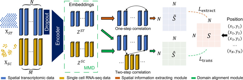
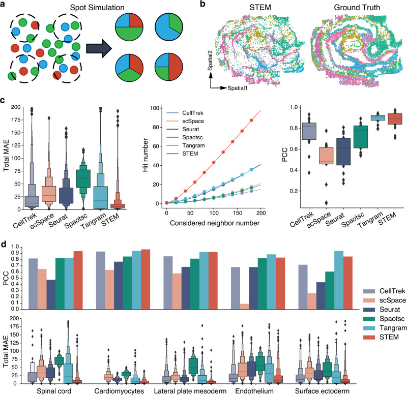
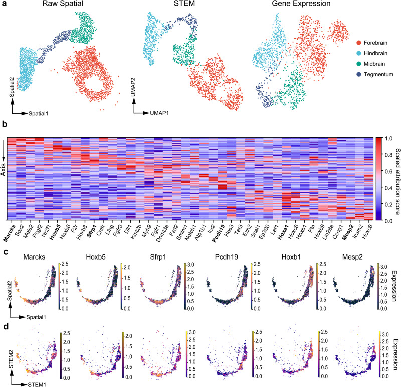
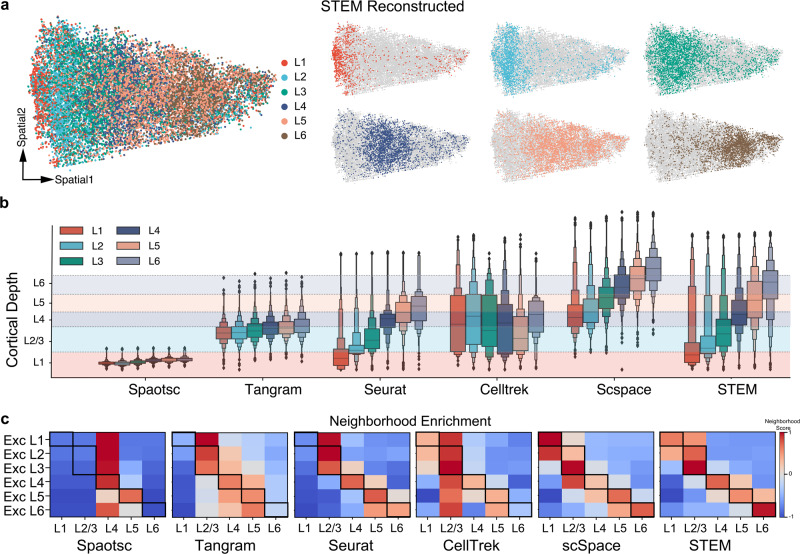
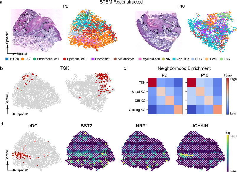
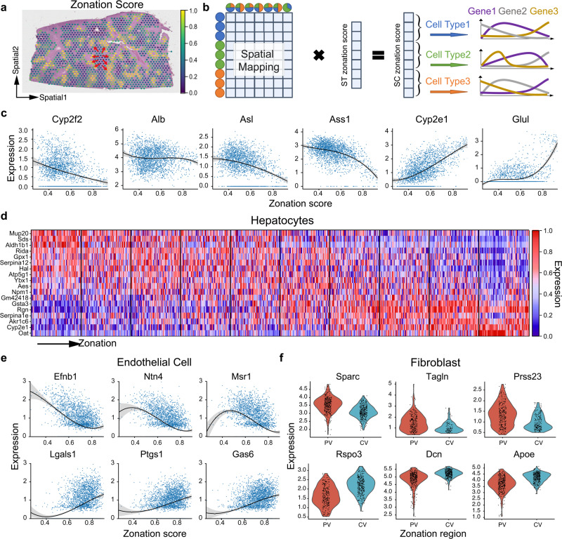
Profiling spatial variations of cellular composition and transcriptomic characteristics is important for understanding the physiology and pathology of tissues. Spatial transcriptomics (ST) data depict spatial gene expression but the currently dominating high-throughput technology is yet not at single-cell resolution. Single-cell RNA-sequencing (SC) data provide high-throughput transcriptomic information at the single-cell level but lack spatial information. Integrating these two types of data would be ideal for revealing transcriptomic landscapes at single-cell resolution. We develop the method STEM (SpaTially aware EMbedding) for this purpose. It uses deep transfer learning to encode both ST and SC data into a unified spatially aware embedding space, and then uses the embeddings to infer SC-ST mapping and predict pseudo-spatial adjacency between cells in SC data. Semi-simulation and real data experiments verify that the embeddings preserved spatial information and eliminated technical biases between SC and ST data. We apply STEM to human squamous cell carcinoma and hepatic lobule datasets to uncover the localization of rare cell types and reveal cell-type-specific gene expression variation along a spatial axis. STEM is powerful for mapping SC and ST data to build single-cell level spatial transcriptomic landscapes, and can provide mechanistic insights into the spatial heterogeneity and microenvironments of tissues.

Fig. 1. Schematic overview of STEM.

Denoting SC and ST gene expression matrices as $X_{ST}\in {\mathbb{R}}^{N\times H}$ and $X_{SC}\in {\mathbb{R}}^{M\times H}$, where $N$ and $M$ are spot and cell numbers, and $H$ is the number of genes. To align the sparsity of the $X_{ST}$ with $X_{SC}$, the $X_{ST}$ first passes through an additional dropout layer. Then the processed ST matrix and the SC matrix pass through a shared encoder of STEM to get the corresponding unified embeddings ${\mathrm{Z}}^{\mathrm{ST}}\in {\mathbb{R}}^{\mathrm{h}}$ and $Z^{SC}\in {\mathbb{R}}^h$ with the same hidden dimension size $h$, respectively. An MMD loss is used to align the distribution of SC and ST embeddings. These embeddings are used to predict the ST-ST spatial adjacency by two modules. The spatial information extracting module uses the correlation between $Z^{ST}$ as the predicted ST-ST adjacency $\tilde{S}\in {\mathbb{R}}^{N\times N}$. The domain alignment module uses the correlation between $Z^{ST}$ and $Z^{SC}$ to create the cross-domain mapping matrices which are multiplied to generate another ST-ST adjacency $\widehat{S}\in {\mathbb{R}}^{N\times N}$. The reconstruction losses $L_{\mathrm{extract}}$ and $L_{\mathrm{trans}}$ between the two predicted adjacency and the ground truth adjacency are computed to optimize the STEM encoder. The ground truth spatial adjacency $S\in {\mathbb{R}}^{N\times N}$ is generated from the spatial coordinate of ST data.

Fig. 2. The performance evaluation results of different methods on a semi-simulation experiment using mouse embryos.

a An illustration of pseudo-ST data generation. Spots on ST data contain only a fraction of single cells. b The reconstructed spatial distribution by STEM versus the ground truth spatial distribution. Colors indicate different cell types or regions. c The mean absolute error (MAE), hit number and Pearson correlation coefficient (PCC) performance of different methods on the first mouse embryo data. The lower the MAE, the better. The higher the hit number and PCC, the better. In PCC results, the two edges of box and horizontal bar inside the box represent the interquartile and median of all values, respectively. d The PCC and MSE performance of methods on five cell types. These manually selected cell types covered all comparison results (equal, lower and higher) between the PCC of Tangram and STEM. The bar plot shows the PCC between ground truth and predicted spatial distributions of five cell types. In MAE results, we used an enhanced boxplot to show more quintiles. The horizontal bar inside the box represents the median of all values. Each edge of the box represents the half percentiles of the rest data, in other words, splitting the rest data into two halves.

Fig. 3. Interpretation of the STEM model.

a Raw spatial distribution of cells and UMAP visualization of cell embeddings obtained from STEM and Gene expression. The color indicates the different spatial region annotation. b The heatmap shows the attribution score of SDGs along the spinal axis. Each column represents a gene expression vector, with the attribution score scaled from 0 to 1. c The ground truth spatial expression patterns of six SDGs. d The STEM reconstructed spatial expression patterns of six SDGs. The genes are highly attributed in different regions, corresponding to the bolder name in the heatmap.

Fig. 4. Performance evaluation on human MTG using all methods.

a The overall reconstructed spatial distribution of single cells obtained by STEM. The six subplots show the spatial distribution of cells in L1-L6 groups. These groups were determined based on tissue dissection information. b Comparison of cortical-depth distribution of cell groups between different methods. The enhanced boxplot in various colors displays the cortical-depth distribution of different single cell groups. The dashed lines indicate the boundaries of layer regions given by ST data. The horizontal bar inside the box represents the median of all values. Each edge of the box represents the half percentiles of the rest data, in other words, splitting the rest data into two halves. c Neighborhood enrichment analysis between SC and ST data using all methods. The x axis represents regions in the ST data while the y axis represents SC excitatory neurons from different dissection layers. The score is row-normalized, and the red color indicates a higher neighborhood score. Bold squares represent areas where high scores are expected.

Fig. 5. STEM results on human squamous cell carcinoma data.

a The HE images and spatial reconstruction results of STEM on patient 2 and patient 10. The black dashed line annotates the tumor-non tumor leading edge observed in the image. The colors of dots represent different cell types. b Highlighted spatial distribution of TSK cells on P2 and P10 slides. c Neighborhood enrichment analysis on tumor keratinocyte subtypes. The score is row normalized and thus asymmetric. Color in red indicates a higher neighborhood score. d The spatial distribution of pDC cells and three spatial expression patterns of corresponding pDC and other immune-related marker genes.

Fig. 6. Cell-type-specific transcriptomic variation along the liver zonation revealed by STEM.

a Distribution of zonation scores on the ST data. A high score indicates the CV region, while a low score indicates the PV region. Arrow in red indicates the direction from a low (PV) to a high (CV) zonation score region. b Illustration of the transfer of zonation scores from ST to SC data. The zonation scores of SC data are obtained by multiplying the SC-ST mapping matrix with the ST zonation score vector. Then cells are grouped into different cell types, and the analysis of cell-type-specific gene variation along the axis can be performed. c Expression profiles of six zonation landmark genes along the PV-CV axis. The x axis represents the zonation score, and the y-axis represents the gene’s raw count expression level. Each curve was obtained by fitting the polynomial function of degree 3 on the corresponding expression value. d Heatmap of the top significantly differentially expressed genes along the PV-CV axis. Gene expression values are scaled, with red indicating high expression and blue indicating low expression. e Expression profiles of six endothelial cell-specific marker genes along the PV-CV axis. The top and bottom genes are highly expressed in the PV and CV regions, respectively. The shading shows the 95 confidence interval. f Violin plots of fibroblast-specific marker genes identified by STEM. The top panel shows the PV marker gene, while the bottom panel shows the CV marker gene.

References

1. Larsson L, Frisén J, Lundeberg J. Spatially resolved transcriptomics adds a new dimension to genomics. Nat. Methods. 2021;18:15–18. doi: 10.1038/s41592-020-01038-7. - DOI - PubMed
1. Palla G, Fischer DS, Regev A, Theis FJ. Spatial components of molecular tissue biology. Nat. Biotechnol. 2022;40:308–318. doi: 10.1038/s41587-021-01182-1. - DOI - PubMed
1. Marx V. Method of the Year: spatially resolved transcriptomics. Nat. Methods. 2021;18:9–14. doi: 10.1038/s41592-020-01033-y. - DOI - PubMed
1. Zhang L, et al. Clinical and translational values of spatial transcriptomics. Signal Transduct. Target. Ther. 2022;7:111. doi: 10.1038/s41392-022-00960-w. - DOI - PMC - PubMed
1. Walker BL, Cang Z, Ren H, Bourgain-Chang E, Nie Q. Deciphering tissue structure and function using spatial transcriptomics. Commun. Biol. 2022;5:220. doi: 10.1038/s42003-022-03175-5. - DOI - PMC - PubMed
Publication types