Substantial kelp detritus exported beyond the continental shelf by dense shelf water transport

Abstract

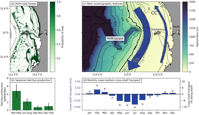
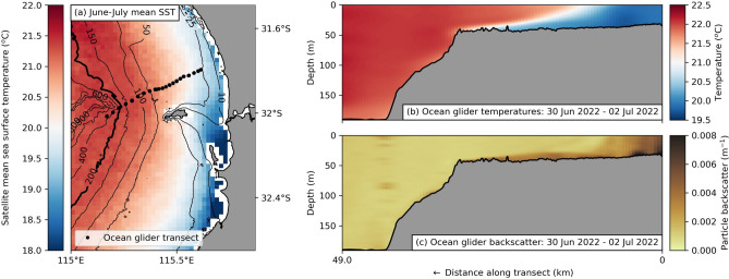
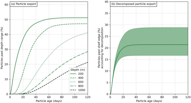
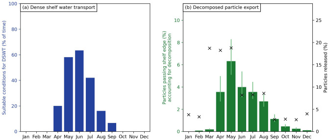
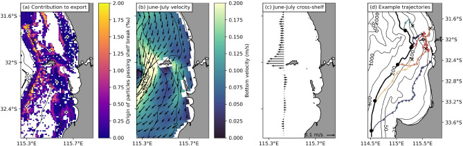
Kelp forests may contribute substantially to ocean carbon sequestration, mainly through transporting kelp carbon away from the coast and into the deep sea. However, it is not clear if and how kelp detritus is transported across the continental shelf. Dense shelf water transport (DSWT) is associated with offshore flows along the seabed and provides an effective mechanism for cross-shelf transport. In this study, we determine how effective DSWT is in exporting kelp detritus beyond the continental shelf edge, by considering the transport of simulated sinking kelp detritus from a region of Australia's Great Southern Reef. We show that DSWT is the main mechanism that transports simulated kelp detritus past the continental shelf edge, and that export is negligible when DSWT does not occur. We find that 51% per year of simulated kelp detritus is transported past the continental shelf edge, or 17-29% when accounting for decomposition while in transit across the shelf. This is substantially more than initial global estimates. Because DSWT occurs in many mid-latitude locations around the world, where kelp forests are also most productive, export of kelp carbon from the coast could be considerably larger than initially expected.

Figure 1

Overview of the Wadjemup continental shelf (WCS) region. (a) Map showing the probability of kelp in the Perth region (see “Methods” section). (b) Seasonal variation of kelp detritus production, based on data from de Bettignies et al.. (c) Map showing the main topological and oceanographic features of the WCS region. Background colors show the bathymetry based on data from Geoscience Australia, with the 200 m depth contour highlighted as the continental shelf edge. The Perth Canyon is located west of Wadjemup. A schematic representation of the southwards flowing Leeuwin Current (LC) and the northwards flowing Capes Current (CC) are shown in blue arrows. The LC is the predominant ocean surface current and extends to approximately 200 m depth. The CC is seasonal and driven by strong southerly seabreezes in the warmer months. (d) Monthly mean bottom cross-shelf transport along the 100 m depth contour (defined as being directed perpendicular to the depth contour), based on CWA-ROMS data for 2017 and averaged over the bottom three model layers. Negative values indicate transport away from the coast and towards the open ocean, and positive values indicate transport towards the coast. Blue bars show the monthly mean bottom cross-shelf velocities in m/s (between 0.002 and 0.03 m/s), black crosses indicate the cross-shelf velocity as a percentage of the monthly mean bottom along-shelf velocity (between 2 and 17% of the mean along-shelf velocity, which itself is between 0.08 and 0.2 m/s). Note that the velocities shown here are used to illustrate the seasonal mean cross-shelf bottom dynamics but are not used to derive any results.

Figure 2

Dense shelf water transport (DSWT) suitable conditions during winter cooling and transects of a DSWT event. (a) Mean sea surface temperature during June and July from 2012–2022 using the gridded, multi-sensor, multi-swath day and night monthly averaged AVHRR IMOS-GHRSST L3S dataset. A band of cooler water along the coast during these months enables the formation of DSWT. Ocean glider measurements from IMOS along a transect (shown with black dots in (a)) during a mission from the 30th of June until the 2nd of July 2022, showing: (b) ocean temperatures; and (c) backscatter (a proxy for suspended matter) during a dense shelf water transport event. Note that the backscatter measures all suspended matter and is likely a mixture between sediment and organic material (including kelp detritus). It is shown here to illustrate the potential for DSWT to transport suspended material across the continental shelf, but is not used to measure the transport of kelp detritus.

Figure 3

Near-bed density maps of simulated (non-decomposing) kelp detritus during peak detrital production months released from the Perth region (Fig. 1a) at the end of: (a) March, one of the hottest months of the year; (b) May, when cooler weather begins; and (c) July, one of the coldest and wettest months of the year. The thick black 200 m contour line highlights the continental shelf edge. During March hardly any simulated detritus was transported past the continental shelf edge. In contrast, during the cooler months of May and July, when dense shelf water transport occurred, simulated detritus was consistently transported past the shelf edge.

Figure 4

Export of simulated kelp detritus for a full year. (a) Percentage of (non-decomposing) kelp detritus exported past different depth ranges from 200 m (continental shelf edge) up to 1000 m as a function of the detritus’ age after being released into the coastal ocean environment. (b) Percentage of detritus exported past the continental shelf edge at 200 m, when accounting for the decomposition of kelp detritus while in transit along the shelf. The dark green line shows the export percentage based on the mean decomposition rate determined by Simpkins et al.. The lighter green band around this line shows the result for the mean ± one standard deviation of the decomposition rate.

Figure 5

Monthly variation in environmental conditions suitable for dense shelf water transport (DSWT) and exported simulated kelp detritus. (a) Suitable environmental conditions for the formation of DSWT, as a percentage of time for each month (see Fig. S8 for a breakdown of the different conditions required for DSWT to form). (b) Percentage of total decomposing kelp detritus exported past the continental shelf edge per month (green bars), compared to the percentage of detritus released each month in our simulation (black crosses). Note that the sum of the monthly percentages adds up to the export percentage for a full year of 21%.

Figure 6

Spatial variation of the export of simulated kelp detritus, ocean bottom currents, and offshore transport. (a) Contribution of different kelp reefs to the export of decomposing detritus past the continental shelf edge, shown per thousand per 0.01°pixel. This figure combines information based on the amount of simulated kelp detritus released per pixel (Fig. S10b), which depends on the probability of kelp (Fig. S10a, Fig. 1a); the amount of simulated kelp detritus that is transported past the shelf edge per pixel (Fig. S10c); and, by accounting for decomposition, how long it takes simulated kelp detritus to make it past the shelf edge per pixel (Fig. S10d). Map of the June and July 2017 mean bottom velocities from the CWA-ROMS model: (b) spatial variation; and (c) cross-shelf transport component only (taken along the 100 m depth contour, and defined as being directed perpendicular to the depth contour, as in Fig. 1d). (d) Example trajectories of simulated kelp detritus transported past the continental shelf edge (black dot indicates where each particle crosses the shelf) released from six different locations (black crosses, also shown in panel (a)). The trajectories shown are those of particles that took the median time to cross the continental shelf edge of all particles that were transported past the shelf edge from that pixel (trajectories of particles that took the shortest and longest time are shown in Fig. S12a,b respectively). The dots on each trajectory are spaced 1 day apart to give an indication of how fast particles were moving in each location.

References

1. Lee, H. et al. Synthesis report of the IPCC sixth assessment report (ar6). In Tech. Rep., Intergovernmental Panel on Climate Change. https://www.ipcc.ch/report/ar6/syr/ (2023).
1. Canadell, J. et al.Climate Change 2021: The Physical Science Basis. Contribution of Working Group I to the Sixth Assessment Report of the Intergovernmental Panel on Climate Change, Chap. Global Carbon and Other Biogeochemical Cycles and Feedbacks 673–816 (Cambridge University Press, 2021).
1. Blue carbon: The role of healthy oceans in binding carbon. In Tech. Rep., United Nations Environment Programme. https://wedocs.unep.org/20.500.11822/7772 (2009).
1. Griscom B, et al. Natural climate solutions. Proc. Natl. Acad. Sci. 2017;114:11645–11650. doi: 10.1073/pnas.1710465114. - DOI - PMC - PubMed
1. Macreadie P, et al. Blue carbon as a natural climate solution. Nat. Rev. Earth Environ. 2021;2:826–839. doi: 10.1038/s43017-021-00224-1. - DOI