Ultrasound Shear Elastography With Expanded Bandwidth (USEWEB): A Novel Method for 2D Shear Phase Velocity Imaging of Soft Tissues

Abstract

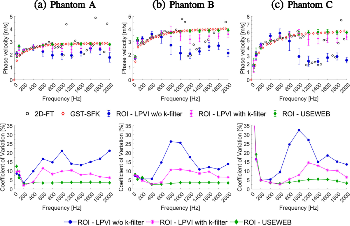
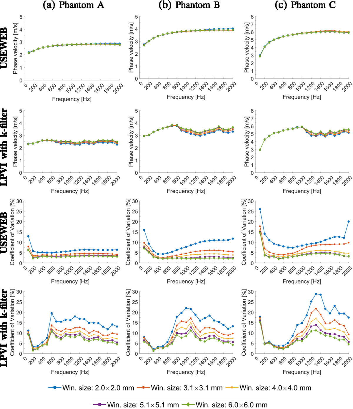
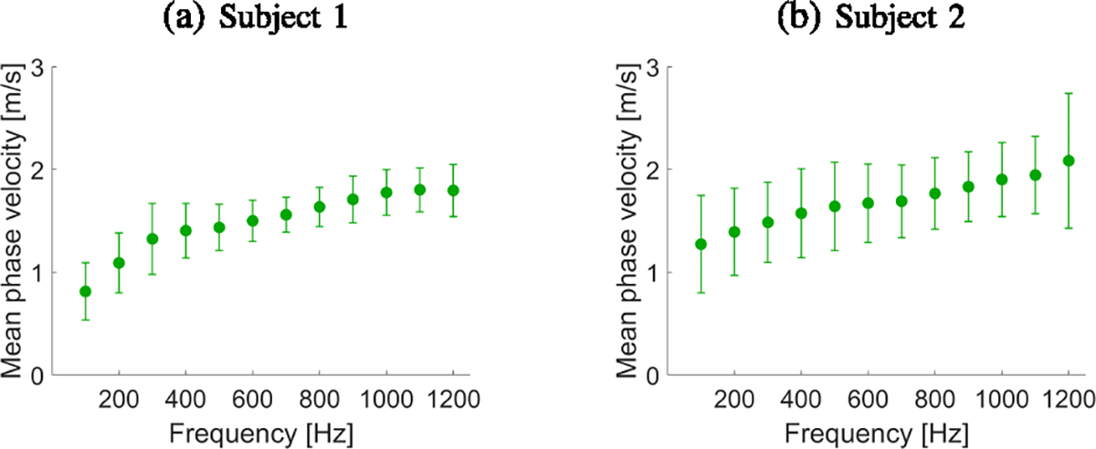
Ultrasound shear wave elastography (SWE) is a noninvasive approach for evaluating mechanical properties of soft tissues. In SWE either group velocity measured in the time-domain or phase velocity measured in the frequency-domain can be reported. Frequency-domain methods have the advantage over time-domain methods in providing a response for a specific frequency, while time-domain methods average the wave velocity over the entire frequency band. Current frequency-domain approaches struggle to reconstruct SWE images over full frequency bandwidth. This is especially important in the case of viscoelastic tissues, where tissue viscoelasticity is often studied by analyzing the shear wave phase velocity dispersion. For characterizing cancerous lesions, it has been shown that considerable biases can occur with group velocity-based measurements. However, using phase velocities at higher frequencies can provide more accurate evaluations. In this paper, we propose a new method called Ultrasound Shear Elastography with Expanded Bandwidth (USEWEB) used for two-dimensional (2D) shear wave phase velocity imaging. We tested the USEWEB method on data from homogeneous tissue-mimicking liver fibrosis phantoms, custom-made viscoelastic phantom measurements, phantoms with cylindrical inclusions experiments, and in vivo renal transplants scanned with a clinical scanner. We compared results from the USEWEB method with a Local Phase Velocity Imaging (LPVI) approach over a wide frequency range, i.e., up to 200-2000 Hz. Tests carried out revealed that the USEWEB approach provides 2D phase velocity images with a coefficient of variation below 5% over a wider frequency band for smaller processing window size in comparison to LPVI, especially in viscoelastic materials. In addition, USEWEB can produce correct phase velocity images for much higher frequencies, up to 1800 Hz, compared to LPVI, which can be used to characterize viscoelastic materials and elastic inclusions.

Fig. 1.

Flowchart of the proposed USEWEB approach. The principal steps of the USEWEB can be summarized as follows: (I) Acquire a 3D shear wave velocity data. (II) Apply directional filter to the data and/or band-pass filter in a wavenumber domain (k-filter) if necessary. (III) Transform 3D spatiotemporal data into 4D time-frequency-space-space domain ($t,f,z,x$) using Eq. (1). (IV) Choose the spectrum at a particular frequency $f_0$. (V) Search for a maximum amplitude of $\mathrm{\Lambda }\left(k_z,k_x,u\right)$ over all steering group velocities, $u$, to obtain the frequency-wavenumber pairs $K$ ($k_z,k_x,f_0$), using Eq. (6). (VI) Calculate spatial distribution of the phase velocity of the shear wave motion for the specified frequency.

Fig. 2.

2D shear wave phase velocity images for the liver fibrosis tissue mimicking homogeneous phantoms with Young’s modulus (E) of 10, 25 and 45 kPa, respectively. The images were calculated for a constant spatial window dimension of 4.47 × 4.47 mm. Phase velocity images were calculated based on the USEWEB and LPVI with k-filter approaches for various, selected frequencies (a) 400, (b) 800, (c) 1200, and (d) 1600 Hz, respectively. Dashed lines present a ROI selected for mean and standard deviation values calculations.

Fig. 3.

Dispersion phase velocity curves (top row) calculated for the liver fibrosis tissue mimicking homogeneous phantoms using the 2D-FT (black circles), GST-SFK (red diamonds) methods for the focal depth of 20 mm, and mean and standard deviation of the phase velocity for LPVI w/o k-filter (blue circles), LPVI with k-filter (magenta stars) and USEWEB (green diamonds). Corresponding coefficient of variation values, CV = SD/MEAN·100%, for reconstructed images are presented in the bottom row. The mean and standard deviation were calculated for ROIs presented in Fig. 2.

Fig. 4.

Mean phase velocity calculated for the liver fibrosis tissue mimicking homogeneous phantoms using the USEWEB and LPVI with k-filter methods, for various frequencies and the spatial window dimensions are shown in the first and second rows, respectively. Corresponding coefficient of variation values, CV = SD/MEAN・100%, for reconstructed images are presented in the third and fourth rows. The mean and CV were calculated for ROIs presented in Fig. 2.

Fig. 5.

2D shear wave phase velocity images for the tissue mimicking viscoelastic phantoms A-C. The images were calculated for a constant spatial window dimension of 4.47 × 4.47 mm. Phase velocity images were calculated based on the USEWEB and LPVI with k-filter approaches for selected frequencies (a) 400, (b) 800, (c) 1200, and (d) 1600 Hz, respectively. Dashed lines present a ROI selected for mean and standard deviation values calculations.

Fig. 6.

Dispersion phase velocity curves (top row) calculated for the tissue mimicking viscoelastic phantoms A-C using the 2D-FT (black circles), GST-SFK (red diamonds) methods for the focal depth of 20 mm, and mean and standard deviation of the phase velocity for LPVI w/o k-filter (blue circles), LPVI with k-filter (magenta stars) and USEWEB (green diamonds). Corresponding coefficient of variation values, CV = SD/MEAN·100%, for reconstructed images are presented in the bottom row. The mean and standard deviation were calculated for ROIs presented in Fig. 5.

Fig. 7.

Mean phase velocity calculated for the tissue mimicking viscoelastic phantoms A-C using the USEWEB and LPVI with k-filter methods, for various frequencies and the spatial window dimensions are shown in the first and second rows, respectively. Corresponding coefficient of variation values, CV = SD/MEAN·100%, for reconstructed images are presented in the third and fourth rows. The mean and CV were calculated for ROIs presented in Fig. 5.

Fig. 8.

2D shear wave phase velocity images, reconstructed for the inclusion size of 6.49 mm, calculated for a constant spatial window dimension of 2.31 × 2.31 mm and various, selected frequencies from (a) 400 Hz to (h) 1800 Hz, respectively. Presented images are computed for the CIRS phantom with an inclusion Type IV, calculated based on the USEWEB (top row) and LPVI with k-filter (bottom row) approaches. Dashed circular lines present a true inclusion location estimated from B-mode. The dashed rectangular box in (a) represents the area utilized for the contrast-to-noise ratio (CNR) calculations in Fig. 10.

Fig. 9.

Horizontal cross-section profiles at the central depth of the 6.49 mm inclusion for the CIRS phantom shown in Fig. 8. The results are plotted for various window dimensions, (a)-(f), and selected frequencies of 400, 800, 1200, and 1600 Hz, for the USEWEB (top row) and LPVI with k-filter (bottom row) approaches, respectively. The horizontal, dash-dotted line corresponds to the nominal phase velocity value provided by the manufacturer. The vertical, dotted lines represent a true inclusion location, and the shaded area corresponds to the width of the spatial window used in that location.

Fig. 10.

(a) Mean phase velocity calculated for the CIRS phantom with an inclusion Type IV and the size of 6.49 mm using the USEWEB and LPVI with k-filter methods, respectively, for various frequencies and the spatial window dimensions. Corresponding contrast-to-noise ratio (CNR), for reconstructed images are presented in (b). The mean and CNR were calculated for ROIs presented in Fig. 8. The horizontal dashed line in (a) corresponds to the nominal phase velocity value provided by the manufacturer.

Fig. 11.

2D shear wave phase velocity images, reconstructed for the inclusion size of 4.05 mm, calculated for a constant spatial window dimension of 1.39 × 1.39 mm and various, selected frequencies from (a) 400 Hz to (h) 1800 Hz, respectively. Presented images are computed for the CIRS phantom with an inclusion Type IV, calculated based on the USEWEB (top row) and LPVI with k-filter (bottom row) approaches. Dashed circular lines present a true inclusion location estimated from B-mode.

Fig. 12.

B-mode images for the in vivo renal transplant data, for (a) Subject 1 and (b) Subject 2.

Fig. 13.

2D shear wave phase velocity images reconstructed in the kidney cortex using the USEWEB method for selected frequencies from 100 Hz to 1200 Hz with an interval of 100 Hz are shown in figures (a)-(l), respectively. The images were calculated for a constant spatial window dimension of 3.10 × 3.10 mm. Dashed lines present manually selected locations of the cortex estimated from B-mode images in Fig. 12.

Fig. 14.

Dispersion phase velocity curves calculated for the in vivo renal transplants using the mean and standard deviation of the phase velocity for USEWEB presented in Fig. 13. The results were calculated for selected ROIs (renal cortex) presented in Fig. 13c.

Fig. 15.

(a) Shear wave velocity motion data. The frequency-wavenumber (f-k) distribution reconstructed based on the (b) 2D-FT, and (c) GST-SFK methods. The f-k maps are normalized by wavenumber maxima in the frequency direction individually for each frequency to show the data optimally. Results were calculated for the experimental, custom-made TM elastic phantoms with E = 10, 25, and 45 kPa, and viscoelastic phantoms A, B, and C.

References

1. Bercoff J, Tanter M, and Fink M, “Supersonic shear imaging: A new technique for soft tissue elasticity mapping,” IEEE Trans. Ultrason., Ferroelectr., Freq. Control, vol. 51, no. 4, pp. 396–409, Apr. 2004. - PubMed
1. Song P, Zhao H, Manduca A, Urban MW, Greenleaf JF, and Chen S, “Comb-push ultrasound shear elastography (CUSE): A novel method for two-dimensional shear elasticity imaging of soft tissues,” IEEE Trans. Med. Imag, vol. 31, no. 9, pp. 1821–1832, Sep. 2012. - PMC - PubMed
1. Sarvazyan A, Hall TJ, Urban MW, Fatemi M, Aglyamov SR, and Garra B, “Elasticity imaging—An emerging branch of medical imaging. An overview,” Current Meds. Imag. Rev, vol. 7, no. 4, pp. 255–282, 2011. - PMC - PubMed
1. Bota S et al., “Meta-analysis: ARFI elastography versus transient elastography for the evaluation of liver fibrosis,” Liver Int, vol. 33, no. 8, pp. 1138–1147, Sep. 2013. - PubMed
1. Sebag F et al., “Shear wave elastography: A new ultrasound imaging mode for the differential diagnosis of benign and malignant thyroid nodules,” J. Clin. Endocrinol. Metabolism, vol. 95, no. 12, pp. 5281–5288, 2010. - PubMed
Publication types