Distributional reinforcement learning in prefrontal cortex

Abstract

The prefrontal cortex is crucial for learning and decision-making. Classic reinforcement learning (RL) theories center on learning the expectation of potential rewarding outcomes and explain a wealth of neural data in the prefrontal cortex. Distributional RL, on the other hand, learns the full distribution of rewarding outcomes and better explains dopamine responses. In the present study, we show that distributional RL also better explains macaque anterior cingulate cortex neuronal responses, suggesting that it is a common mechanism for reward-guided learning.

Fig. 1. Diverse optimism in value coding across ACC neurons.

a, Top, on each trial, subjects chose between two cues of neighboring probability value. Bottom, each probability value could be denoted by two stimuli, resulting in two stimulus sets (see ref. for task details). b, Example responses from three separate neurons demonstrating different levels of optimism. In each plot the mean firing rate is plotted as a function of time and split according to the chosen value (probability) level. There are four chosen values (0.3–0.9 probability) because subjects rarely chose the 0.1 probability level (choice accuracy was at ceiling: 98%). Insets demonstrate that the firing rate is a nonlinear function of value. Mean firing rate (z-scored across trials) in a 200- to 600-ms window after cue onset is plotted as a function of the four values. Reversal points are the interpolated values at which there is 0 change from the mean firing rate, an index of nonlinearity. Shaded regions and error bars denote s.e.m. c, Histogram showing a diversity of reversal points across ACC RPE-coding neurons. Coloring denotes optimism as defined by reversal point, with red being more optimistic. d, Scatter plot showing reversal points estimated in half of the data strongly predicted those in the other half. Each point denotes a neuron. Inset, log(P values) of Pearson’s correlation between 1,000 different random splits of the data into independent partitions. Across partitions, the mean R = 0.44 and geometric mean of the P values was P = 0.003 (black line). Bootstrapping to obtain a summary P value was also significant (P < 0.01). e, Scatter plot showing reversal points estimated in stimulus set 1 strongly predicted those in stimulus set 2 (R = 0.41, P = 0.009). Each point denotes a neuron. f, AP topographic location of the neuron predicted its reversal point, with more anterior ACC neurons being more optimistic (R = 0.37, P = 0.016). As we had two independent noisy measures of each neuron’s optimism (reversal point and asymmetry; Fig. 2), we used the mean of the two measures (after z-scoring them), which we call ‘neuron optimism’. Neuron optimism is plotted against the normalized AP locations within ACC. The normalization ensures that, for example, the most anterior portion of the ACC in one animal corresponds to that in the other. Each point denotes a neuron. See Extended Data Fig. 6 for further analyses.

Fig. 2. Diverse asymmetric scaling of RPEs predicts optimism.

a, An example neuron’s responses at each of the task epochs: choice, feedback on rewarded trials and feedback on unrewarded trials. β⁺ and β⁻ are betas corresponding to the scaling of positive and negative RPEs. Betas are calculated on the mean firing rate in a 200- to 600-ms window after feedback. Error bars denote s.e.m. Note that, for rewarded and unrewarded trials, we do not display the lowest and highest value levels, respectively, owing to a small number of trials giving unreliable traces. b, Histogram showing a diversity of asymmetric scaling across ACC RPE neurons. Coloring denotes optimism as defined by asymmetric scaling, with red more optimistic. c, Same format as Fig. 1d but for asymmetric scaling consistency: mean R = 0.32, P = 0.014 across data partitions. Each point denotes a neuron. d, Asymmetric scaling estimated at feedback predicted reversal point at choice: R = 0.41, P = 0.0079. Each point denotes a neuron.

Fig. 3. Diverse asymmetric learning.

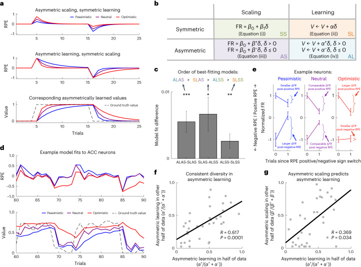
a,b, Asymmetric scaling and asymmetric learning are both predictions of distributional RL, but are dissociable. Asymmetric scaling reflects differences in the degree to which positive and negative RPEs are scaled to predict firing rate. Asymmetric learning reflects differences in the rate of state value update after positive and negative RPEs (which may or may not be affected by asymmetric scaling). These different learning rates are denoted by α⁺ and α⁻, respectively. $\delta =r-V$ is the RPE, where r is the reward on the current trial and V the value. a, Simulated examples demonstrating the difference between asymmetric scaling and learning, as governed by the equations in b. The top shows predicted RPEs generated by asymmetric scaling with symmetric learning (equations (iii) and (ii)). In this extreme case, the scaling does not impact learning and the learned value would converge on the expectation. The middle and bottom show the converse: RPEs and corresponding values generated by symmetric scaling with asymmetric learning (equations (i) and (iv)). We have presented them in this way to highlight how asymmetric scaling and asymmetric learning can be dissociable phenomena that we can measure separately, not because we do not predict that they are related. On the contrary, we show that they are related in g. c, Comparing the crossvalidated model fits revealed that a model with both asymmetric learning and asymmetric scaling (ALAS) is the best explanation of the ACC data, and the fully classic (symmetric) model (SLSS) is the worst model of the data. Each bar in the bar graph shows the comparison between a pair of models and is the difference in the R² value of the two models being compared. Error bars denote s.e.m. The significance of the differences is determined by paired, two-sided Student’s t-tests over neurons: ^*P ≤ 0.05, ^**P ≤ 0.01, ^***P ≤ 0.001. d, Example model fits. Top, RPE regressors generated using learning rate parameters fitted to individual neuron data, for three different neurons from the same session. Different levels of optimism can be seen via the different rates at which RPEs tend back toward zero after changes in state value (denoted by the dashed black line in the bottom plot). Bottom, this is reflected in the corresponding values. The pessimistic neuron (shown in blue), for example, is quick to devalue but slow to value. e, Example real neuron responses around transitions in the sign of the RPE, from three separate neurons. We used the best-fitting model to define trials when the RPE switched from negative to positive, or vice versa. We then plotted the mean firing rate on that first trial of the switch and the subsequent trial, and observed asymmetries in the rate of change in the firing rate after the first positive versus negative RPE, as predicted by distributional RL in a. For example, the (pessimistic) neuron on the left changes its firing rate more following negative than positive RPEs (the slope for negative RPEs is more positive than the slope for positive RPEs is negative), indicating that it has learnt more from negative than from positive RPEs. The converse pattern is true for the (optimistic) neuron on the right. Error bars denote s.e.m. f, The per-neuron asymmetry in learning derived from the model, defined as ${\alpha }^{+}/\left({\alpha }^{+}+{\alpha }^{-}\right)$, estimated in one half of the data predicted that in the other half of the data (R = 0.62, P = 0.0001), demonstrating that there is consistent diversity in asymmetric learning across the population of neurons, as predicted by distributional RL. g, Asymmetric learning and asymmetric scaling positively correlated, consistent with the theoretical proposal that asymmetric scaling drives asymmetric learning (R = 0.35, P = 0.04 for a correlation between asymmetric learning estimated in the first data partition and asymmetric scaling estimated in the second, and R = 0.38, P = 0.03 for the converse correlation; average across partitions: mean R = 0.37, geometric mean P = 0.03).

Extended Data Fig. 1. Timeseries demonstrating value-related variance.

The mean across neurons of the coefficient of partial determination (CPD) for value (cued probability) over time, following cue onset. The CPD measures how much variance in each neuron’s firing is explained by a given regressor (see below). This timeseries validates the 200–600 ms post-onset window that we used in order to match that used in Dabney, Kurth-Nelson et al., because that window very closely matches the peak value-related coding in the timeseries (as in Kennerley et al.). We therefore used 200–600 ms and did not try any other time windows in order to avoid any possible p-hacking. Nonetheless we note that in a window that captures this peak, defined as when the CPD is higher than two thirds of the maximum CPD (270–620 ms), the core correlation between reversal point and asymmetric scaling was significant, R = 0.38, P = 0.019. Shaded region is the SEM across neurons. Note, as in Kennerley et al., the CPD for regressor X_i is defined by ${\mathit{CPD}(X}_i)=\left[\mathit{SSE}\left(X_{-i}\right)-\mathit{SSE}\left(X_{-i},X_i\right)\right]/\mathit{SSE}\left(X_{-i}\right)$, where SSE(X) is the sum of squared errors in a regression model that includes a set of regressors X, and $X_{-i}$ is a set of all the regressors included in the model except X_i. The CPD for X_i is more positive if X_i explains more variance in neuronal firing.

Extended Data Fig. 2. Reason for Z-scoring to fit the reversal points.

a–c) Three example neurons’ firing rate plotted as a function of time since cue onset, and split according to the four value levels, showing that some neurons increase their firing relative to baseline pre-stimulus firing rate for all reward levels (a), others increase or decrease it depending on the reward level (b) and others decrease it for all reward levels (c). Shaded regions denote SEM. The reason for Z-scoring in our data is as follows. In dopamine neurons, it appears that any firing rate deviation from baseline activity (that is, pre-stimulus onset activity) is signalling a reward prediction error. This is not true for cortical neurons, which may, for example, increase (as in a) or decrease (c) their firing to all reward levels. If this is the case, then deviation from baseline cannot be assumed to denote an RPE. That some neurons either increase or decrease their firing to all reward levels is indicative of the heterogenous coding schemes evident in PFC neurons. Given this, we can isolate the component of the activity that is associated with RPE by calculating z-scores, and using deviation from mean firing to capture the same effect and compute reversal points. Therefore our reversal point measure captures, for each neuron, the relative differences in responses to different reward levels (that is, the non-linearity) that indicates optimism, rather than being affected by overall shifts in firing. These reversal points, that is, the value at which the neuron firing reverses from below to above the mean firing in the epoch, are an index of neuron optimism; the higher the reversal point, the more optimistic the neuron, and neurons with reversal points above 2.5 are optimistic and below 2.5 are pessimistic (Methods).

Extended Data Fig. 3. Results hold with a different measure of non-linearity at choice.

a) Histogram showing diverse quadratic betas. b) Histogram showing the log p-values for consistency of these quadratic betas across partitions and the corresponding geometric mean. c) Pearson correlation between asymmetric scaling and quadratic betas.

Extended Data Fig. 4. Simultaneous diversity within session.

Four simultaneously recorded cells from the session with most reward-sensitive cells (9 in total), demonstrates there is diversity in optimism even within a session. Across cells, responses to middle value levels are both above and below the linear interpolation between lowest and highest values’ responses. Mean normalised firing is plotted for each of the 4 value levels. Error bars denote SEM. Firing rates are normalised such that responses to value 1 and 4 have mean firing rate 0 and 1, respectively. Normalisation allows comparison across cells of responses to middle value levels. Responses to value 2 across the 9 simultaneously recorded cells were significantly diverse; ANOVA rejected the null hypothesis that across cells the value 2 responses were drawn from the same mean (F(8,405) = 3.56, P = 0.0005). The same was true for responses to value 3 (F(8,441) = 2.16, P = 0.0291). This diversity was also present when including all cells in the analysis (value 2: F(40,1658) = 3.82, P = 2.74 × 10⁻¹⁴, and value 3: F(40,1842) = 4.73, P = 4.99 × 10⁻²⁰), and in individual subjects (first animal: value 2; F(11,516) = 3.18, P = 0.0006, value 3; F(10,520) = 3.61, P = 0.0001; second animal: value 2; F(29,1142) = 3.92, P = 2.6 × 10⁻¹¹ value 3; F(29,1322) = 5.47, P = 1.7 × 10⁻¹⁸).

Extended Data Fig. 5. Lack of diversity in OFC and LPFC.

We additionally ran analyses in all reward selective neurons (as opposed to only RPE-selective neurons) in OFC and LPFC as an exploratory analysis to assess whether consistent diversity was present when more neurons entered the analysis, since these regions have a smaller proportion of RPE-selective neurons compared to ACC. Same analysis as in Fig. 1, but for OFC and LPFC on all reward-selective neurons or RPE selective neurons. We applied exactly the same criteria and analyses to these brain regions as we did in ACC. As in Fig. 1, we computed the Pearson correlation for each of 1000 independent data partitions, and calculate the mean and geometric mean of the R and p-values, respectively. The coloured (left) histograms are the distributions of the reversal points, and the grey (right) histograms are the log(p-values) from the correlations. a) OFC reward-selective neurons. b) OFC RPE-selective neurons. c) LPFC reward-selective neurons. d) LPFC RPE-selective neurons. With the exception of the reward-selective neurons in OFC (a), none of these analyses were significant. Moreover, when we compared the diversity of these reward-selective neurons in OFC (a) across stimulus set (that is, Fig. 1e analysis), the correlation between stimulus set 1 and 2 was not significant (R = 0.15; P = 0.35). This may suggest the diversity in these OFC neurons is due to, for example, stimulus-selectivity, whereby some neurons are selective for stimuli coding the edges of the reward distribution, which could appear as optimism/pessimism in a given stimulus set, but does not generalise across stimulus set as would be expected from diversity related to value. The RPE-selective neurons had no consistent diversity, and as RPE selectivity is a requirement to test further predictions of distributional RL, we did not look for further distributional RL signatures in these brain regions.

Extended Data Fig. 6. Anatomical gradient in a different subset of probability selective neurons.

Here we test for the anatomical gradient across those neurons that were probability selective at choice, but did not meet the criteria for RPEs. This analysis is to test the robustness of the gradient result by assessing whether it replicates in an independent set of neurons. The neuron optimism of these neurons is measured using the reversal point. We present this data here to supplement the gradient analyses in Fig. 1, but note that it is less clear what the predictions of distributional RL are for these non-RPE neurons, and so it is unclear exactly what the reversal point means in these neurons. Nevertheless we present this result to demonstrate the gradient of the reversal point measure replicates in an independent set of neurons (R = 0.28, P = 0.013, by Pearson correlation).

Extended Data Fig. 7. Other brain regions demonstrate some or no evidence for distributional RL.

Same format and analyses as Fig. 3c in the main text, and Extended Data Fig. 8. We repeated our model comparison analyses in the other brain regions recorded in this task. These regions are also known to contain reward and prediction error signals, and so we may expect them to carry signatures of distributional RL. We found evidence for distributional RL in caudate (a; n = 26 neurons), weak evidence for it in dorsolateral prefrontal cortex (b; n = 39), and no evidence for it in putamen (c; n = 34). Error bars denote SEM. *P ≤ 0.05, **P ≤ 0.01, ***P ≤ 0.001. However we note that, similar to the first dataset presented in this manuscript, the number of selective neurons in these other regions is smaller than in ACC (which had 94 out of 240 neurons selective; 39%); caudate had 26 out of 115 neurons (23%), dorsolateral prefrontal cortex had 39 out of 187 neurons (21%), and putamen had 34 out of 119 neurons (29%). Furthermore, there were too few neurons selective under the stricter criteria for defining RPE-selective neurons (from Bayer & Glimcher 2005 and used in other parts of this manuscript; Methods), and so we do not analyse the model comparisons in these regions further; caudate (9 out of 115 neurons; 8%), dorsolateral prefrontal cortex (7 out of 187 neurons; 4%), and putamen (11 out of 119 neurons; 9%). We therefore do not wish to make claims about the presence or absence of distributional RL in these regions; rather it is possible the lack of strong evidence for distributional RL in these regions arises from a smaller proportion of neurons that are encoding RPEs.

Extended Data Fig. 8. All pairwise model comparisons for asymmetric learning and scaling analyses.

Same format as Fig. 3 in the main text. a) Bar graphs with all 6 pairwise model comparisons for the 94 neurons defined as selective using the RPE regressors from Miranda et al. (Methods). ALAS – SLAS, SLAS – ALSS, and ALSS – SLSS are the same as in the main text. *P ≤ 0.05, **P ≤ 0.01, ***P ≤ 0.001. b) Same as A but for only those neurons (n = 33) that meet a strict definition for being RPE selective. That is, as defined in Bayer & Glimcher 2005, those neurons that encode reward on the current trial and previous trial but with opposite signs (see Methods for further details).

Extended Data Fig. 9. Results are very similar when taking the linear parameters β₀ and β₁ across cross-validated partitions.

Same format as Fig. 3 in the main text. In the main text analyses, we re-fit the linear parameters β₀ and β₁ in the test data during cross-validation. As explained in the Methods, this is to isolate our analysis to the asymmetries in scaling, rather than the analysis being impacted by, for example, overall (non-asymmetric) gain. Here we show the same result as in Fig. 3c in the same 94 neurons, but when carrying over the linear parameters (β₀ and β₁) as well as the asymmetric parameters (S, α⁺ and α−) to predict firing rate, and therefore do not re-estimate the linear parameters in the test data. We find that the pattern of results remains the same. Error bars denote SEM. *P ≤ 0.05, **P ≤ 0.01, ***P ≤ 0.001.

Extended Data Fig. 10. Alternative model agnostic, directly data-derived, measures of asymmetric learning correlate with model fit parameter-derived asymmetric learning.

a) Similar to the analysis in Fig. 3e, wherein we analysed the neural firing rates around transitions in the sign of the RPE (as defined from the best-fitting model), we also analysed firing rates on the first and second trials following the highest reward option and the lowest reward option (that is, analogous to Fig. 3e but where the x-axis is trial number following the onset of consecutive trials of highest – or lowest – reward level delivered). On these trial types we can be confident that all neurons (regardless of optimism) will have positive and negative RPEs, respectively (because these reward levels are at the extremes of the reward distribution). We observed diversity across the population of neurons in a per-neuron t-score measure, obtained from an unpaired t-test testing for differences in firing rate change between the first and second trial following a high reward vs. the same following a low reward. (Note this is the same measure that we used in the main text to provide a per-neuron measure capturing the asymmetries plotted in Fig. 3e, which we correlated with model-derived asymmetric learning.) These t-scores reflect the per-cell significance in rejecting the null hypothesis that there is no difference in firing rate change from the first to second trial receiving highest reward, vs. that on lowest reward. a is a histogram of these t-scores, and demonstrates there is significant diversity across the population. b) This t-score measure in a correlated across neurons with asymmetric learning derived from the best-fitting model (R = 0.21, P = 0.044). c) Additionally, we constructed a regression model to capture asymmetries in the effect of a highest vs. lowest reward level delivered on the previous trial on the current trial’s firing rate. This also captures asymmetries in learning. The regression model was the following: $FR={\beta }_0+{\beta }_{1}Rew\left(t\right)+{\beta }_{2}HighestRew\left(t-1\right)+{\beta }_{3}LowestRew\left(t-1\right)$, where Rew(t) is the reward on the current trial, HighestRew(t−1) is a binary regressor with value 1 if the previous trial delivered the highest reward level and 0 otherwise, and LowestRew(t−1) is similarly a binary regressor with value 1 if the previous trial delivered a lowest reward level and 0 otherwise. We then do a [1 -1] contrast for β₃ vs. β₂ to capture differences in the effect of a highest vs. lowest reward delivered on the previous trial on the current trial’s firing rate. This value will be more positive if delivery of the highest reward level on the previous trial decreases the firing on the current trial more than delivery of the lowest reward level increases it (this pattern would be expected from an optimistic neuron). Delivery of the highest reward level is expected to decrease firing on the subsequent trial (captured by β₂) due to the learning induced from positive outcomes: it should suppress subsequent RPEs as the value expectation is now higher (same logic as in Bayer & Glimcher). Similarly, delivery of the lowest reward level is expected to increase firing on the subsequent trial (captured by β₃) due to the learning induced from negative outcomes: it should increase subsequent RPEs as the value expectation is now lower. The [1 -1] contrast testing β₃ vs. β₂ captures the relative differences in these effects and is therefore another index of asymmetric learning: optimistic neurons should be more impacted by the highest reward level compared to the lowest. We found the t-scores of this contrast were also diverse across the population (c), correlated with the other data-driven measure described above in a and b (d; R = 0.44, P < 0.001), and also correlated with asymmetric learning derived from the best-fitting model (e; R = 0.21, P = 0.039). Combining both of these noisy measures from a and c into a hybrid measure (by averaging the t-scores) gives a summary model-agnostic measure that is also correlated with model-derived asymmetric learning: R = 0.25, P = 0.016.