Elevated genetic risk for multiple sclerosis emerged in steppe pastoralist populations

Abstract

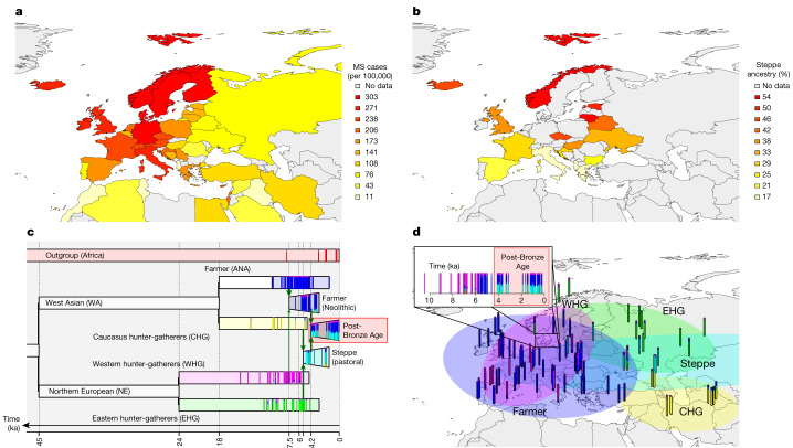
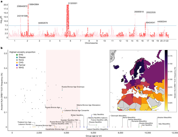
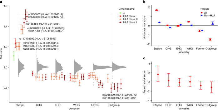
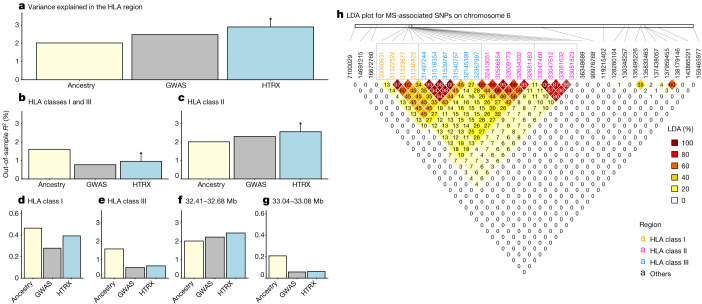
Multiple sclerosis (MS) is a neuro-inflammatory and neurodegenerative disease that is most prevalent in Northern Europe. Although it is known that inherited risk for MS is located within or in close proximity to immune-related genes, it is unknown when, where and how this genetic risk originated¹. Here, by using a large ancient genome dataset from the Mesolithic period to the Bronze Age², along with new Medieval and post-Medieval genomes, we show that the genetic risk for MS rose among pastoralists from the Pontic steppe and was brought into Europe by the Yamnaya-related migration approximately 5,000 years ago. We further show that these MS-associated immunogenetic variants underwent positive selection both within the steppe population and later in Europe, probably driven by pathogenic challenges coinciding with changes in diet, lifestyle and population density. This study highlights the critical importance of the Neolithic period and Bronze Age as determinants of modern immune responses and their subsequent effect on the risk of developing MS in a changing environment.

Fig. 1. The population history of Europe is associated with the modern-day distribution of MS.

a, The modern-day geographical distribution of MS in Europe. Prevalence data for MS (cases per 100,000) were obtained from ref. . b, Steppe ancestry in modern samples as estimated by ref. . c,d, A model of European prehistory onto which our reference samples were projected using non-negative least squares (NNLS) for population painting (see Methods) (c) and the same data represented spatially (d). Samples are shown as vertical bars representing their ‘admixture estimate’ obtained by NNLS (see Methods) from six ancestries: EHG (green), WHG (pink), CHG (yellow), farmer (ANA + Neolithic; blue), steppe (cyan) or an outgroup (represented by ancient Africans; red). Important population expansions are shown as growing bars, and ‘recent’ (post-Bronze Age) non-reference admixed populations are shown for the Denmark time transect (see Extended Data Fig. 2 for details). Chronologically, WHG and EHG were largely replaced by farmers amid demographic changes during the ‘Neolithic transition’ around 9,000 years ago. Later migrations during the Bronze Age about 5,000 years ago brought a roughly equal steppe ancestry component from the Pontic-Caspian steppe to Europe, an ancestry descended from the EHG from the middle Don River region and the CHG. Steppe ancestry has been associated with the Yamnaya culture and then with the expansion westwards of the Corded Ware culture and Bell Beaker culture, with eastward expansion in the form of the Afanasievo culture^,. ka, thousand years ago.

Fig. 2. Areas of unusual local ancestry in the genome and ancient and modern frequencies of HLA-DRB1*15:01.

a, Local ancestry anomaly score measuring the difference between the local ancestry and the genome-wide average (capped at –log₁₀(P) = 20; Methods). Significant peaks (reaching genome-wide significance P < 5 × 10^–8, two-tailed t test before adjustment for multiple testing, as shown by the blue horizontal line) are labelled with chromosome position (build GRCh37/hg19). b, HLA-DRB1*15:01 frequency (y axis) in ancient populations over time (x axis; yr bp, years before the present); this is the highest effect variant for MS risk (calculated using the rs3135388 tag SNP). For each ancestry (CHG, EHG, WHG, farmer, steppe), the five populations with the highest amount of that ancestry are labelled; other populations are shown as grey points. HLA-DRB1*15:01 was present in one sample before the steppe expansion but rose to high frequency during the Yamnaya formation (approximate time period shaded red). The geographical distribution of HLA-DRB1*15:01 frequency in modern populations from the UK Biobank is also shown (inset; grey represents no data). FBC, funnel beaker culture; LBK, linear pottery culture (Linearbandkeramik); CWC, corded ware culture.

Fig. 3. Associations between local ancestry at fine-mapped MS-associated SNPs and MS in a modern population.

a, Risk ratio of SNPs for MS based on WAP (see Methods) when decomposed by inferred ancestry. The mean and s.d. were calculated for each ancestry on the basis of bootstrap resampling for each chromosome (n = 408,884 individuals). The distribution of risk ratios for each ancestry is shown as a raincloud plot. SNPs significant at the 1% level are shown individually, coloured by chromosome or HLA region, and those with a risk ratio of >1.2 or <0.8 are annotated with their rsID, HLA region and position (build GRCh37/hg19). b,c, ARS (see Methods) for MS. The mean and confidence intervals were estimated by either bootstrapping over individuals (b; which can be interpreted as testing the power to reject a null hypothesis of no association between MS and ancestry; n = 1,000 bootstrap resamples with replacement over 24,000 individuals) or bootstrapping over SNPs (c; which can be interpreted as testing whether ancestry is associated with MS across the genome; n = 1,000 bootstrap resamples with replacement over 204 SNPs). We show the results for all associated SNPs (red) and non-HLA SNPs only (blue) when bootstrapping over individuals.

Fig. 4. MS association in the HLA region.

a–g, Comparison of variance explained in MS within the UK Biobank for all fine-mapped HLA SNPs with an independent contribution. The plots compare GWAS (treating SNPs as having independent effects), local ancestry at the SNPs and HTRX (haplotypes), after accounting for covariates (Methods), for fine-mapped MS-associated SNPs in the HLA region (a), the HLA class I and class III regions (b), the HLA class II region (c), the HLA class I region (d), the HLA class III region (e) and subregions of the HLA class II region chosen from LD (f,g). Upward-pointing arrows for HTRX indicate where the values are lower bounds (Methods). h, Genetic correlations in the HLA region at our time depth from ancestry-based LD (LDA;  Methods; see Supplementary Fig. 50 for LD).

Fig. 5. Evidence for selection on MS-associated SNPs.

a, Stacked line plot of the pan-ancestry PALM analysis for MS, showing the contribution of SNPs to disease risk over time. SNPs are shown as stacked lines, with the width of each line proportional to the population frequency of the positive risk allele, weighted by its effect size. When a line widens over time, the positive risk allele has increased in frequency, and vice versa. SNPs are sorted by the magnitude and direction of selection, with positively selected SNPs at the top, negatively selected SNPs at the bottom and neutral SNPs in the middle. SNPs are coloured by their corresponding P value in a single-locus selection test. The asterisk marks the Bonferroni-corrected significance threshold, and nominally significant SNPs are shown in yellow and labelled by their rsID. SNPs marked with the dagger symbol are located in the HLA locus. The y axis shows the scaled average PRS in the population, ranging from 0 to 1, with 1 corresponding to the maximum possible average PRS (that is, when all individuals in the population are homozygous for all positive risk alleles), and the x axis shows time in units of thousands of years before the present. SE, standard error. b, Maximum-likelihood trajectories for four SNPs tagging HLA-DRB1*15:01, for all ancestry paths combined (All) and for each path separately (Extended Data Fig. 1 and Methods). Portions of the trajectories with high uncertainty (that is, posterior density of <0.08) have been masked. The background is shaded for the approximate time period in which the ancestry existed as an actual population. The y axis shows the derived allele frequency (DAF), and the x axis shows time in units of thousands of years before the present.

Extended Data Fig. 1. Methods map detailing datasets used, methods, and statistics.

A narrative of the evidence used is provided in the centre, with boxes on each side detailing the methods used. Boxes are coloured by the dataset used.

Extended Data Fig. 2. Ancient sample PCA, map, ancestry proportions through time for samples in Denmark.

(1) PC1 vs PC2 of the filtered Western Eurasian ancient samples included in this study. Black circled points are Danish Medieval and post-Medieval samples published here for the first time. Major component ancestry locations are labelled. (2) Map of ancient filtered Eurasian and African ancient samples included in this study. (3a) Map of reference data and time transect of Denmark as in Fig. 1. (3b) More recent ancient data (samples <4,200 years ago) not used as reference, showing the clines of the main ancestry components from (3a).

Extended Data Fig. 3. LDAS on chromosome 2 and 6.

LDA score is a) high in the LCT/MCM6 region while it is b) low in the HLA region.

Extended Data Fig. 4. Signatures of selection at the HLA locus showing different regions of the HLA (horizontal coloured bar) and locations of MS-associated SNPs (vertical lines, coloured by the variance explained by 6 ancestries).

a): Whole Chromosome 6 “local ancestry” decomposition by genetic position. b). HLA “local ancestry” decomposition by genetic position. c): LDA score; low values are indicative of selection for multiple linked loci, while high values indicate positive selection. d): pi scores (nucleotide diversity) for CEU (Northern and Western European ancestry). MS-associated SNPs fall in highly diverse regions of the HLA. e): Fst scores (divergence between two populations) for CEU vs YRI(Yoruba); locally higher scores indicate regions that have undergone differential selection between the two populations.

Extended Data Fig. 5. The number of protective associations with pathogens or infectious diseases for the MS- and RA-associated selected SNPs.

The number of protective associations to specific pathogens and/or diseases associated with the MS- and RA-SNPs that showed statistically significant evidence for selection using CLUES. One SNP can have a link to more than one pathogen and/or disease (see ST11 and ST12 for details on each SNP). Eight and twenty SNPs had no detectable links to any pathogen or infectious disease in the MS and RA SNP sets, respectively.

Extended Data Fig. 6. Evidence for selection on RA-associated SNPs.

a) Stacked line plot of the pan-ancestry PALM analysis for RA, showing the contribution of SNPs to disease risk over time. SNPs are shown as stacked lines, the width of each line being proportional to the population frequency of the positive risk allele, weighted by its effect size. When a line widens over time the positive risk allele has increased in frequency, and vice versa. SNPs are sorted by the magnitude and direction of selection, with positively selected SNPs at the top, negatively selected SNPs at the bottom, and neutral SNPs in the middle. SNPs are coloured by their corresponding p-value in a single locus selection test. The asterisk marks the Bonferroni corrected significance threshold, and nominally significant SNPs are shown in yellow and labelled by their rsIDs. SNPs marked with the dagger symbol are located in the HLA locus. The Y-axis shows the scaled average polygenic risk score (PRS) in the population, ranging from 0 to 1, with 1 corresponding to the maximum possible average PRS (i.e. when all individuals in the population are homozygous for all positive risk alleles) and the X-axis shows time in units of thousands of years before present (kyr BP). b) Posterior likelihood trajectory for rs660895, tagging HLA-DRB1*04:01, inferred by CLUES. Statistical significance was assessed by applying a Bonferroni correction for the number of tests performed for each trait.

Extended Data Fig. 7. Associations between local ancestry at fine-mapped RA SNPs and RA in a modern population.

a) Risk ratio of SNPs for RA based on weighted average prevalence (WAP; see Methods), when decomposed by inferred ancestry. A mean and standard deviation are calculated for each ancestry based on bootstrap resampling, for each chromosome (n = 408,884 individuals). The distribution of risk ratios at each ancestry is shown as a raincloud plot. SNPs significant at the 1% level are shown individually, coloured by chromosome or HLA region, and those with risk ratio >1.1 or <0.9 are annotated with rsID, HLA region and position (build GRCh37/hg19). b-c) Genome-wide Ancestral Risk Scores (ARS, see Methods) for RA. Mean and confidence intervals are estimated by either bootstrapping over individuals (b, which can be interpreted as testing power to reject a null hypothesis of no association between RA and ancestry; n = 1000 bootstrap resamples with replacement over 24,000 individuals) and bootstrapping over SNPs (c, which can be interpreted as testing whether ancestry is associated with RA genome-wide; n = 1000 bootstrap resamples with replacement over 55 SNPs). We show results for all associated SNPs (red) and non-HLA SNPs only (blue) when bootstrapping over individuals.

References

1. Attfield, K. E., Jensen, L. T., Kaufmann, M., Friese, M. A. & Fugger, L. The immunology of multiple sclerosis. Nat. Rev. Immunol.10.1038/s41577-022-00718-z (2022). - PubMed
1. Allentoft, M. E. et al. Population genomics of post-glacial western Eurasia. Nature10.1038/s41586-023-06865-0 (2024). - PMC - PubMed
1. Walton C, et al. Rising prevalence of multiple sclerosis worldwide: insights from the Atlas of MS, third edition. Mult. Scler. J. 2020;26:1816–1821. doi: 10.1177/1352458520970841. - DOI - PMC - PubMed
1. International Multiple Sclerosis Genetics Consortium et al. Multiple sclerosis genomic map implicates peripheral immune cells and microglia in susceptibility. Science. 2019;365:eaav7188. doi: 10.1126/science.aav7188. - DOI - PMC - PubMed
1. Bjornevik K, et al. Longitudinal analysis reveals high prevalence of Epstein–Barr virus associated with multiple sclerosis. Science. 2022;375:296–301. doi: 10.1126/science.abj8222. - DOI - PubMed