Achieving ultra-low and -uniform residual magnetic fields in a very large magnetically shielded room for fundamental physics experiments

Abstract

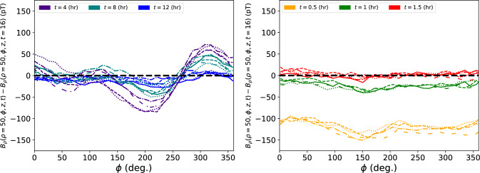
High-precision searches for an electric dipole moment of the neutron (nEDM) require stable and uniform magnetic field environments. We present the recent achievements of degaussing and equilibrating the magnetically shielded room (MSR) for the n2EDM experiment at the Paul Scherrer Institute. We present the final degaussing configuration that will be used for n2EDM after numerous studies. The optimized procedure results in a residual magnetic field that has been reduced by a factor of two. The ultra-low field is achieved with the full magnetic-field-coil system, and a large vacuum vessel installed, both in the MSR. In the inner volume of $\sim 1.4{\text{m}}^3$, the field is now more uniform and below 300 pT. In addition, the procedure is faster and dissipates less heat into the magnetic environment, which in turn, reduces its thermal relaxation time from $12\text{h}$ down to $1.5\text{h}$.

Fig. 1

Arrangement of the degaussing coils, which produce flux around the z-axis on MSR layer 6 drawn as a cube box. The yellow square represents the access door. Label A (green): corner coils similar on all layers; Label B (red): additional coils only on layer 6; Label C (purple): additional smaller coils only on the layer 6 door. The blue arrows indicate the direction of the magnetic flux $\mathrm{\Phi }$ produced inside the shielding material by a current through the indicated coils

Fig. 2

Scheme of the electrical connections from the DACs to the degaussing coils of layer 1. The relays K0.1 to K0.4 are the main switches, which can connect the supply rails “supply A” and “supply B” in either polarity to the power amplifier. The relays K1.1 to K1.3 are used to connect the degaussing coils of layer 1 to the supply rails, selecting which of the x-, y-, and z-degaussing coil is supplied with current. In order to activate the return path for layer 1, K1.0 is closed. In the idle state when the layer one coil is not powered, all K1 relays are open. Identical schemes are used for layers 2 to 5

Fig. 3

The scheme of the relay connections for layer 6 is more elaborate then for the other layers. It enables connection to any of the three coils in series with arbitrary relative polarity. The signal always goes from the rails supply A to supply B (see Fig. 2). The relays K6.10, K6.20, and K6.30 select which coils are not powered by providing a current path that bypasses the coil. The hardware (using relay logic) does not permit all three of those relays to close simultaneously, avoiding a short circuit. When K6.10 is open, two of the relays K6.11 to K6.14 are closed in order to select in which polarity the current runs though the x degaussing coil of layer 6. The same scheme is used to power independently the y and z coils. In the idle state when the layer 6 coil is not powered all K6 relays are open

Fig. 4

Visualization of magnetic flux across the surface of layer 6 during a simultaneous excitation of x, y,  and z coils, when the coils are connected with the sign combination $x_{+}{y}_{-}{z}_{+}$. The arrows indicate the flux direction inside the walls for a positive half-wave of the degaussing function. The dotted line indicates the corner axis around which the flux is generated. Here, the axis definition matches Fig. 1, where the red surface has the access door (again yellow)

Fig. 5

Voltage monitoring of the Rohrer amplifier output as a function of time with a linear increase/decrease of amplitude. The zoomed inset shows the oscillating behavior. An up-time of $1\text{s}$, hold-time of $1\text{s}$, down-time of $500\text{s}$, and frequency of $5\text{Hz}$ is used

Fig. 6

Voltage output of Rohrer amplifier as a function of current. The upper-left inset figure shows the voltage monitoring as a function of time, similar to Fig. 5, and is linear as the Rohrer is operated in voltage-mode. The different colors highlight which part of the degaussing waveform populates the current–voltage space. The lower-right inset is the same but for current as a function of time. See text for details

Fig. 7

$\varphi$-averaged transverse residual magnetic field, $B_{\perp }$, at $\rho =50$ cm, as a function of z, for the serial degaussing sequence (blue) and the simultaneous degaussing sequence with polarity $x_{+}{y}_{-}{z}_{+}$ (red). The dashed line shows the average field sampled in $\varphi$ at $\rho =50$ cm with fixed z points, and the envelope is $2\sigma$ spread around the average at each z

Fig. 8

Same as Fig. 7 but for the serial degaussing sequence (blue) and the double-simultaneous degaussing sequence with polarity $x_{+}{y}_{-}{z}_{-}$ then $x_{+}{y}_{-}{z}_{+}$ (red)

Fig. 9

Thermal relaxation effect on the residual magnetic field $B_{\rho }$, after a full degaussing. (Left): using the previous sequence, the difference of the magnetic field at various wait times [4 (purple), 8 (teal), and 12 (blue) hours] and the field after 16 h, at $\rho =50$ cm as a function of $\varphi$ for different z positions [(solid): $z=-30$ cm, (dotted): $z=-15$ cm, (dashed): $z=0$ cm, (dotted-dashed): $z=15$ cm, (loosely-dashed): $z=30$ cm]. The different line styles indicate the various z positions sampled. (Right): The same but for the optimized degaussing sequence for wait times [0.5 (yellow), 1.0 (green), and 1.5 (red) hours]. Already after 1.5 h, the field has reached equilibrium with the state after 2 h, and, even initially, the field is much more uniform in $\varphi$. Uncertainty has been omitted for clarity, but the spread in the different lines of the same color give a sense of the field non-uniformity in the precession volume

Fig. 10

Temperature drift after starting a degaussing with the optimized sequence (red) and previous sequence (blue), measured by a thermocouple mounted on the inside of the MSR on layer 6. The solid lines indicate when the degaussing sequence is finished (red at $\sim 2.5\text{h}$ and blue at $\sim 3.5\text{h}$). With the previous sequence, there is a significantly longer decay time until thermal stability ($\sim 12\text{h}$), whereas the new sequence reaches stability in about $1.5\text{h}$ after the degaussing finishes, as supported by Fig. 9

Fig. 11

Average total residual magnetic field $|{\mathbf{B}}_{\text{tot}}(\mathbf{r})|=\sqrt{B_x^2+B_y^2+B_z^2}$, as a function of distance from center of the vacuum tank, for the serial degaussing sequence (blue) and the optimized sequence (red). The envelope is $2\sigma$ of the average field sampled in $|\mathbf{r}|=7\text{cm}$ bins, where the bins are indicated by the horizontal bars. The optimized sequence includes a fluxgate correction for $B_z$ ($\sim$90 pT), where the correction was extracted by rotating the fluxgate 180^∘. The previous sequence (*) did not measure this offset, due to a mechanical issue during the measurement, however the same correction that was extracted in the optimized sequence was applied here as well. This leaves an undetermined offset, added in quadrature, still possible to the blue curve

References

1. Ayres NJ, et al. Eur. Phys. J. C. 2021;81:512. doi: 10.1140/epjc/s10052-021-09298-z. - DOI - PMC - PubMed
1. B. Lauss, B. Blau, SciPost Phys. Proc. 004 (2021)
1. Abel C, et al. Phys. Rev. Lett. 2020;124:081803. doi: 10.1103/PhysRevLett.124.081803. - DOI - PubMed
1. Ramsey NF. Phys. Rev. 1950;78:695. doi: 10.1103/PhysRev.78.695. - DOI
1. Afach S, et al. J. Appl. Phys. 2014;116:084510. doi: 10.1063/1.4894158. - DOI