Improving sub-pixel accuracy in ultrasound localization microscopy using supervised and self-supervised deep learning

Abstract

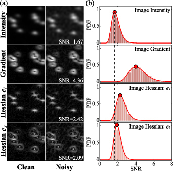
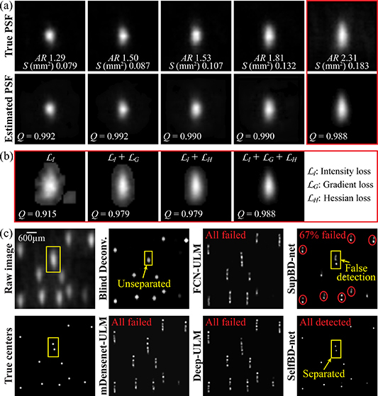
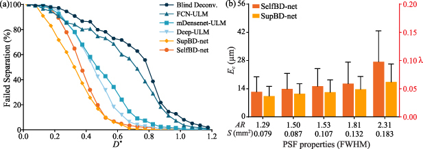
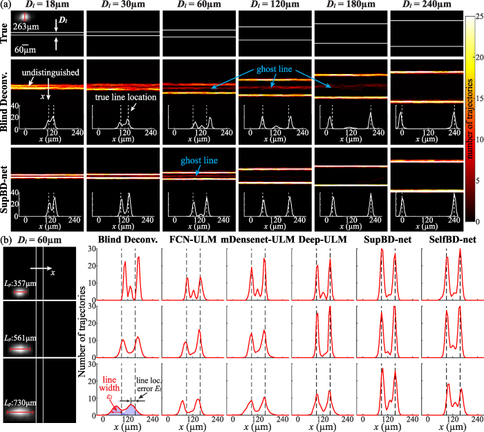
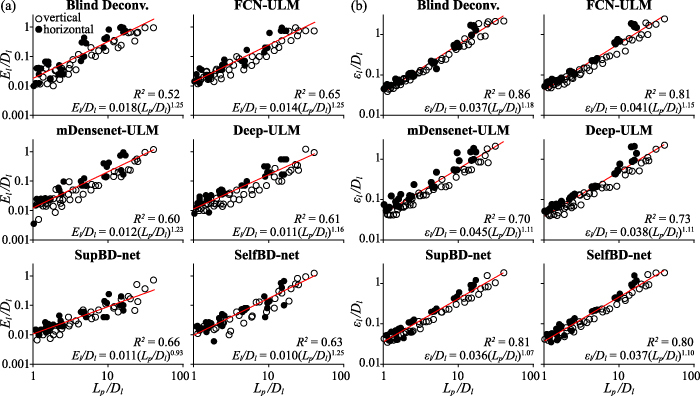
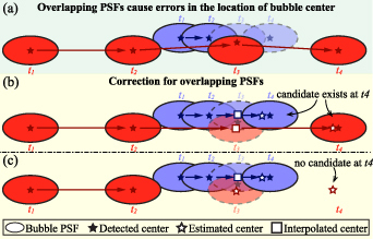
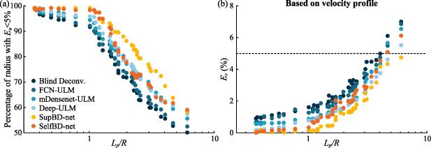
With a spatial resolution of tens of microns, ultrasound localization microscopy (ULM) reconstructs microvascular structures and measures intravascular flows by tracking microbubbles (1-5 μm) in contrast enhanced ultrasound (CEUS) images. Since the size of CEUS bubble traces, e.g. 0.5-1 mm for ultrasound with a wavelength λ = 280 μm, is typically two orders of magnitude larger than the bubble diameter, accurately localizing microbubbles in noisy CEUS data is vital to the fidelity of the ULM results. In this paper, we introduce a residual learning based supervised super-resolution blind deconvolution network (SupBD-net), and a new loss function for a self-supervised blind deconvolution network (SelfBD-net), for detecting bubble centers at a spatial resolution finer than λ/10. Our ultimate purpose is to improve the ability to distinguish closely located microvessels and the accuracy of the velocity profile measurements in macrovessels. Using realistic synthetic data, the performance of these methods is calibrated and compared against several recently introduced deep learning and blind deconvolution techniques. For bubble detection, errors in bubble center location increase with the trace size, noise level, and bubble concentration. For all cases, SupBD-net yields the least error, keeping it below 0.1 λ. For unknown bubble trace morphology, where all the supervised learning methods fail, SelfBD-net can still maintain an error of less than 0.15 λ. SupBD-net also outperforms the other methods in separating closely located bubbles and parallel microvessels. In macrovessels, SupBD-net maintains the least errors in the vessel radius and velocity profile after introducing a procedure that corrects for terminated tracks caused by overlapping traces. Application of these methods is demonstrated by mapping the cerebral microvasculature of a neonatal pig, where neighboring microvessels separated by 0.15 λ can be readily distinguished by SupBD-net and SelfBD-net, but not by the other techniques. Hence, the newly proposed residual learning based methods improve the spatial resolution and accuracy of ULM in micro- and macro-vessels.

Keywords: deep learning; self-supervised learning; super-resolution ultrasound imaging; ultrasound localization microscopy.

Figure 1.

Illustration of the problems in raw CEUS images and sample results of blind deconvolution. (a) A sample raw CEUS image of a porcine’s coronal brain section. A bubble trace (white box) is magnified at the top right to show its millimetric size, which is much larger than its physical size (∼5 μm). A group of closely seated bubbles are marked in the yellow circle showing the difficulty in distinguishing them. Showing in the dashed boxes are the moving interrogation windows used for estimating the local PSF. (b) The corresponding estimated spatial distribution of PSF. Highlighted in the white, yellow, and blue dashed boxes are the PSFs corresponding to the same windows in (a). (c) A sample enhanced image after blind deconvolution.

Figure 2.

A sample procedure for generating the synthetic images. The subarea of a CEUS image containing a similar PSF is demonstrated next to the synthetic data.

Figure 3.

The PDF of the relative RMS intensity difference (E_k ) between the original PSFs and the up- and down- sampled ones.

Figure 4.

An illustration of the network structure of SupBD-net. The current SupBD-net consists of two ConvBlocks, four local residual blocks (ResBlock) along with one global residual block, one transpose convolution layer for upscaling, one final convolution layer for generating 2D images, and a sigmoid layer to ensure a 0–1 intensity range of the output image. The image size × number of feature channels are listed above each block.

Figure 5.

An illustration of the network structure of SelfBD-net. Shown in the top left is an additional network, named k-net, used for estimating the PSF from the raw CEUS image. The k-net and the pretrained x-net are jointly trained on the CEUS images with unknown PSFs using the loss functions provided in the top right.

Figure 6.

Comparison of the signal-to-noise ratio (SNR) for image intensity, gradient, and Hessian. (a) A sample comparison of a clean synthetic CEUS image (left) versus the same one with added noise at a typical level (right). From top to bottom, demonstrated images are image intensity, gradient magnitude, and the magnitudes of the first and second eigenvalues of the image Hessian. The corresponding SNR for the noisy image is listed in the bottom right of each image. (b) The SNR PDF for 2500 noisy synthetic images with a typical bubble density and noise level. The dashed line shows the center SNR level for image intensity, and the red dots show the center SNR level for each class.

Figure 7.

The procedures for training SelfBD-net. (a) Step 1: updating the k-net while freezing the x-net. After 40 iterations, the k-net converges and learns to deform the Gaussian disk to resemble the true PSF shown on the right. (b) Step 2: freezing the k-net and updating layers after the global residual learning in x-net. The first 50 iterations are demonstrated where the false detections (red circle) in the x-net output are gradually removed and the closely seated bubbles (green circle) are separated. The resulting estimated bubble centers are close to the true centers shown on the right.

Figure 8.

Sample images demonstrating the raw synthetic image, true bubble center map, and the center maps obtained based on blind deconvolution, FCN-ULM, mDensenet-ULM, Deep-ULM, and SupBD-net. The scale bar is provided at the bottom right of the raw image.

Figure 9.

Variations of the mean error in the detected bubble center (E_c —bars) and its standard deviation (error bars) with PSF area (S) and aspect ratio (AR) for a single bubble at a peak noise level of 0. The left vertical axis shows values in μm and the right shows values in fractions of wavelength (λ).

Figure 10.

Variations of the mean error in the detected bubble center (E_c —bars) and its standard deviation (error bars) for varying bubble concentrations (columns), peak noise levels (rows), and PSF area and aspect ratio (S and AR, horizontal axis). The left vertical axis shows values in μm and the right shows values in fractions of λ.

Figure 11.

Visualization of the SelfBD-net outputs. (a) A comparison of the true (top row) and the estimated PSFs (bottom row) along with their correlation coefficients (Q). (b) A comparison of the right most PSF in (a) estimated using different loss functions. (c) A sample case comparing the estimated bubble centers of each method. Here, enclosed in the yellow box are two closely seated bubbles that are only correctly distinguished by the SelfBD-net.

Figure 12.

Evaluation of SelfBD-net using vertically oriented PSFs. Variations of E_c (a) and the percentage of falsely detected bubbles (η, (b)) with increasingly elongated PSFs under a bubble concentration of 0.5 mm⁻² and a peak noise level of 0.16. For the PSF with an aspect ratio of 1.81, also shown are the variations of E_c with increasing noise level under a bubble concentration of 0.5 mm⁻² (c) and with increasing bubble concentration under a peak noise of 0.16 (d). For (a), (c), and (d), the left vertical axis shows values in μm and the right in fractions of λ. For (a)–(d), the bar height shows mean values and the error bar shows the standard deviation.

Figure 13.

Evaluation of SelfBD-net using the horizontally oriented PSFs with a bubble concentration of 0.5 mm⁻² and a peak noise level of 0.16. (a) Variations of the percentage of unseparated bubbles with the bubble distance normalized by the PSF FWHM length along the line connecting the two centers (D*). (b) Comparison of E_c between SelfBD-net and SupBD-net for increasing PSF size. The left vertical axis shows values in μm and the right in fractions of λ. The bar height shows mean values and the error bar shows the standard deviation.

Figure 14.

Spatial resolution of closely located parallel lines for different image processing methods. (a) Sample heat maps of bubble trajectories showing the effect of increasing line spacing (D_l ). (b) Sample cross-sectional profiles averaged along the line showing the effect of PSF FWHM length in the direction perpendicular to the line (L_p ). The error in line location (E_l ) and line width (ϵ_l ) are indicated in the bottom left. For (a) and (b), the vertical dashed lines show the true location of each line. The PSF size is not shown on the same scale as the line spacing.

Figure 15.

Variations of nondimensionalized: (a) line location error (E_l/D_l ), and (b) line width (ϵ_l/D_l ) with PSF size (L_p/D_l ). The red line shows the least-square-fitted power law, whose expression as well as the coefficient of determination (R ²) are provided at the bottom of each panel. The solid dots denote data of horizontal lines, and hollow dots represent data of vertical lines.

Figure 16.

Determining the threshold for negligible ghost lines using support vector machine (SVM). (a) Sample illustration of the definition of the parameters, namely, the area fraction, AF, and the normalized index of detection, ID. (b) Scatter plots of AF and ID, as well as the decision boundaries estimated by the SVM. The red dots correspond to ghost lines, the blue dots to primary lines, and the black encircled ones are the support vectors. A few examples are shown on the right side demonstrating cases with negligible ghost lines (cases 1–4), and non-negligible ones (cases 5–8).

Figure 17.

Summarization of the ability of each method to separate closely located parallel lines for different D_l and L_p.

Figure 18.

Correction of the error in velocity measurement caused by falsely detected bubble centers of overlapping PSFs. (a) The bubble-to-track assignment without correction for the overlapping PSFs. Overlapping PSFs correction strategies when a candidate is (b) detected (solid star) and (c) not detected in the vicinity of estimated (hollow star) bubble location at t ₄. For each track, once a candidate is assigned at t ₄, the location for the overlapping PSF at t ₃ is replaced by the interpolated value (hollow box). Otherwise, it is terminated at t ₂.

Figure 19.

(a) Sample SupBD-net results showing velocity profiles at three streamwise locations of bubbles (L_p = 263 μm) traveling inside a horizontal blood vessel (R= 180 μm) measured without correction for overlapping PSFs. The measured values are marked by circles and the prescribed velocity profile is plotted in curves. (b) The corresponding velocity profiles measured with correction. (c) The relative error in velocity (E_u ) measured without (red) and with (blue) correction for the overlapping PSF. Also plotted in black is E_u caused by the error in bubble center detection, i.e. .

Figure 20.

The variations with normalized PSF size L_p/R of: (a) the percentage of the radius with E_u < 5% and (b) the relative error in radius (E_r ) measured based on the velocity profile. The vertical axis is in linear scale while the horizontal axis is in log scale.

Figure 21.

Measurement of the vessel radius based on the profiles of the number of bubble tracks. (a) Gaussian fitting (red curve) to the number of tracks (blue circles) showing inconsistent length which matches the prescribed profile (black curve). (b) The zero crossings of parabolic fitting showing better consistency with the prescribed radius. (c) The variations with L_p/R of E_r measured based on the number of tracks and parabolic fit. The vertical axis is in linear scale while the horizontal axis is in log scale.

Figure 22.

Sample heat maps and velocity distributions of the cortical vasculature in the left cerebral hemisphere of a piglet measured based on the indicated methods. For each panel: top row: heat maps of the number of bubble trajectories; bottom row: corresponding maps of average blood velocity; and middle row: heat maps and velocity distributions in the highlighted magnified subregion enclosed by the white box.

Figure 23.

(a) A magnified view of the region in the blue box of figure 22. Two cross-sectional profiles along four closely spaced microvessels (line 1) and two moderately spaced microvessels (line 2) are provided for all methods to compare the spatial resolution of different methods. (b) A magnified view of the region in the yellow box of figure 22, where the cross-sectional profile along a moderate blood vessel (line 3) is provided for all methods comparing their abilities to estimate the radius of this vessel. The left and right panels show the radius estimation based on the parabolic fit to the number of tracks and velocity profile, respectively.

References

1. Vincent J-L, et al. Clinical review: update on hemodynamic monitoring-a consensus of 16. Crit. Care. 2011;15:1–8. doi: 10.1186/cc10291. - DOI - PMC - PubMed
1. Schinkel A F L, Kaspar M, Staub D. Contrast-enhanced ultrasound: clinical applications in patients with atherosclerosis. Int. J. Cardiovasc. Imaging. 2016;32:35–48. doi: 10.1007/s10554-015-0713-z. - DOI - PMC - PubMed
1. Hwang M. Introduction to contrast-enhanced ultrasound of the brain in neonates and infants: current understanding and future potential. Pediatr. Radiol. 2019;49:254–62. doi: 10.1007/s00247-018-4270-1. - DOI - PMC - PubMed
1. Greis C. Quantitative evaluation of microvascular blood flow by contrast-enhanced ultrasound (CEUS) Clin. Hemorheol. Microcirc. 2011;49:137–49. doi: 10.3233/CH-2011-1464. - DOI - PubMed
1. Crapper M, Bruce T, Gouble C. Flow field visualization of sediment-laden flow using ultrasonic imaging. Dyn. Atmos. Oceans. 2000;31:233–45. doi: 10.1016/S0377-0265(99)00035-4. - DOI
LinkOut - more resources