Spatial analysis of tissue immunity and vascularity by light sheet fluorescence microscopy

Abstract

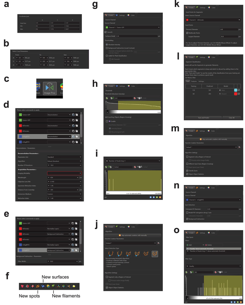
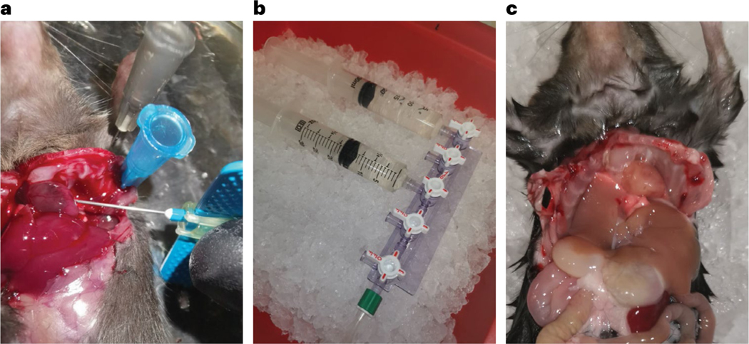
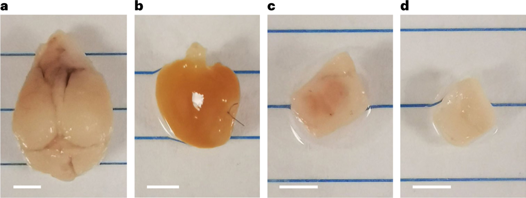
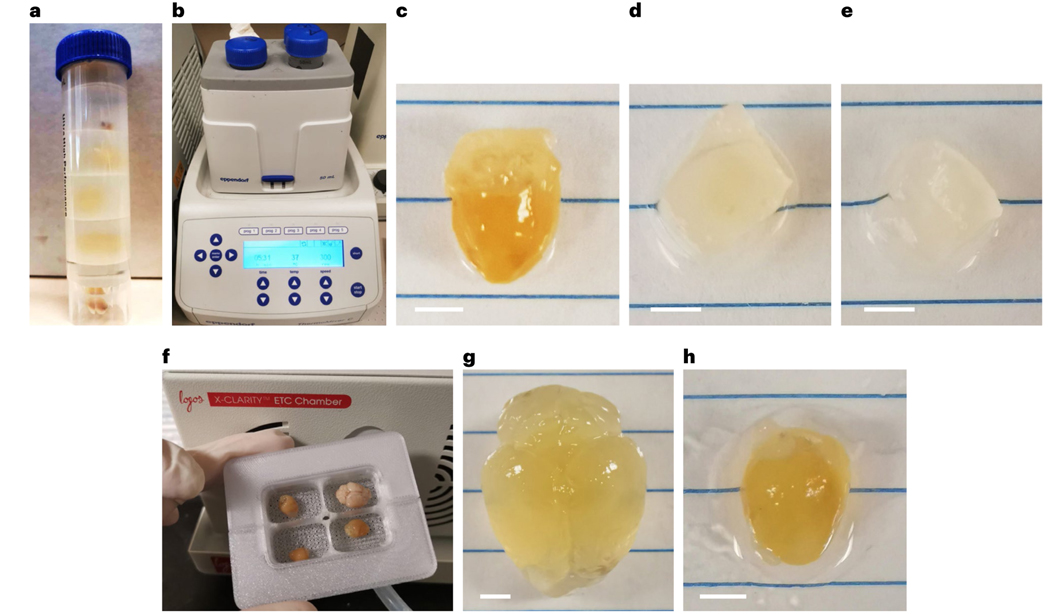
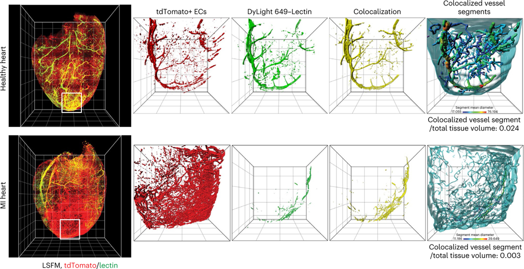
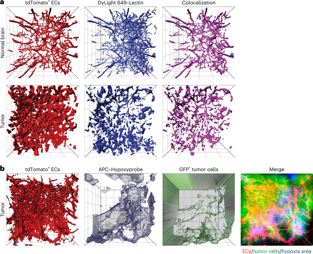
The pathogenesis of cancer and cardiovascular diseases is subjected to spatiotemporal regulation by the tissue microenvironment. Multiplex visualization of the microenvironmental components, including immune cells, vasculature and tissue hypoxia, provides critical information underlying the disease progression and therapy resistance, which is often limited by imaging depth and resolution in large-volume tissues. To this end, light sheet fluorescence microscopy, following tissue clarification and immunostaining, may generate three-dimensional high-resolution images at a whole-organ level. Here we provide a detailed description of light sheet fluorescence microscopy imaging analysis of immune cell composition, vascularization, tissue perfusion and hypoxia in mouse normal brains and hearts, as well as brain tumors. We describe a procedure for visualizing tissue vascularization, perfusion and hypoxia with a transgenic vascular labeling system. We provide the procedures for tissue collection, tissue semi-clearing and immunostaining. We further describe standard methods for analyzing tissue immunity and vascularity. We anticipate that this method will facilitate the spatial illustration of structure and function of the tissue microenvironmental components in cancer and cardiovascular diseases. The procedure requires 1-2 weeks and can be performed by users with expertise in general molecular biology.

Extended Data Fig. 1 |. LSFM analysis of healthy mouse brain left hemisphere.

Healthy Cdh5-Cre^ERT2;LSL-tdTomato mice were perfused with DyLight 649-lectin. Brain tissue was excised, followed by tissue clearing and LSFM imaging. Each minor tick on the grid represents 1 mm.

Extended Data Fig. 2 |. LSFM analysis of tissue samples after long-term storage.

a, GBM was induced in Cdh5-Cre^ERT2;LSL-tdTomato mice, followed by perfused with hypoxyprobe. Tissue samples were subjected to tissue clearing, and stored in RIMS at 4°C for 2.5 years and imaged by LSFM. Each minor tick on the grid represents 1 mm. b, MI was induced in Cdh5-Cre^ERT2;LSL-tdTomato mice, followed by perfused with lectin. Tissue samples were subjected to tissue clearing, and stored in RIMS at 4°C for 2.5 years and imaged by LSFM. Each minor tick on the grid represents 0.5 mm.

Extended Data Fig. 3 |. Key steps of image processing and analysis in Imaris.

a, Voxel size correction in “Image Properties” (Step 42). b, Crop out ROI in “Crop 3D” (Step 43). c, “Image Processing” module (Step 44). d, Setting deconvolution parameters in the “Image Processing” module (Step 44). e, Preprocessing the image using “Normalize Layers” and “Background Subtraction “ (Steps 45, 46). f, Creating objects for feature registration (Step 48). g, Initial parameters for creating surface objects (Step 48A(ii)). h, Thresholding of surface object creation (Step 48A(iii)). i, Filtering generated surface objects by size (Step 48A(iv)). j, Multiscale Points method of generating filament seed points (Step 48B(ii)). k, Seed point filtering by vessel diameter (Step 48B(ii)).l, Segment classification and filtering by machine learning-based model (Step 48B(iii)). m, Initial parameters for creating spot objects (Step 48C(i)). n, Spot detection by feature diameter (Step 48C(ii)). o, Filter Spot feature by quality and diameter/size (Step 48C(iii–iv)).

Fig. 1 |. Overview of the protocol.

Overview of the experimental design involved in this protocol. The procedure is segmented into several essential steps, including animal model preparation for tumor and MI induction, sample preparation, hydrogel polymerization for the preservation of biomolecular structures and functionalities, tissue semi-clearing for removing lipids and making the tissue transparent, sample immunostaining, RI matching and mounting for reducing light scattering and improving image clarity, tissue imaging using LSFM, and data processing and analysis. Figure created with BioRender.com.

Fig. 2 |. Tissue perfusion for sample preparation.

A system for transcardial perfusion. a, A 25 G BD vacutainer needle was inserted into the left ventricle of the heart (Step 6). Mice were imaged before perfusion. b, The perfusion needle was connected to a stopcock manifold with inlets connected to two 30 ml syringes loaded with the respective perfusates (anticoagulant perfusate and AP solution). Perfusates were placed on ice and injected manually by pushing the syringes (Steps 6–7). c, Mice were imaged after perfusion. Successful perfusion can be verified by change in the color of the heart and liver (from bright or dark red to light salmon or yellow) and stiffening of limbic muscles (Step 7).

Fig. 3 |. Sample processing by hydrogel polymerization.

a–d, Samples imaged after hydrogel polymerization (Steps 13–14) for whole-brain tissue with GBM tumor (a), whole-heart tissue with MI (b), trimmed GBM tumor tissue (c) and normal brain tissue (d). Scale bars, 3 mm.

Fig. 4 |. Sample processing by tissue semi-clearing.

a–e, Tissue samples were subjected to passive tissue semi-clearing. Samples were placed in a compartmentalized 50 ml conical tube (a) and incubated in a thermomixer (b) (Step 16A(i)). Normal heart sample with MI was imaged 7 d after semi-clearing (c) (Step 16A(i–iii)). Trimmed GBM tumor (d) and normal brain samples (e) were imaged 4 d after semi-clearing (Step 16A(iii)). f, Tissue samples were subjected to ETC semi-clearing in a polycarbonate 3D-printed ETC tissue holder (Step 16B(i)). g, Healthy whole-brain sample after 1 d ETC (Step 16B(iii)). h, Healthy whole-heart sample after 2 d ETC (Step 16B(iii)). In c–e, g and h, scale bars, 3 mm.

Fig. 5 |. RI matching and sample mounting.

a–c, Tissue samples were processed by RI matching (Step 24). Trimmed healthy brain tissue (a), trimmed GBM tumor tissue (b) and whole-heart tissue (c) were imaged. Dashed lines indicate the edges of tissue samples. Scale bars, 3 mm. d–f, Tissue samples were mounted. Samples were subjected to RIMS–agar encapsulation in trimmed 3 ml syringes (d) (Step 25). Sample blocks were encapsulated on a 3D-printed tissue holder (e) (Steps 26–30). Sample encapsulated in RIMS–agar is fixed to a 3D-printed sample holder by glue (f). g, Encapsulated sample blocks were fixed to a 3D-printed tissue holder, immersed in RIMS (Steps 31–32). Black dashed lines outline sample blocks. Red dashed lines outlines tissue holder.

Fig. 6 |. LSFM analysis for vascular structure and perfusion in hearts.

Heart samples were collected from lectin-perfused healthy or diseased Cdh5–Cre^ERT2; LSL–tdTomato mice 3 weeks post-MI, followed by tissue semi-clearing and LSFM imaging. Left, whole-heart images. Each minor tick on the grid represents 1 mm. White boxes represent the ROI selected for zoomed-in views. Right, zoomed-in view of healthy left ventricle and MI areas. Each minor tick on the grid represents 500 μm. For colocalized vessel segment panels, cyan surface represents actual tissue volume. Registered vessel segments are color coded by mean diameter of the segments.

Fig. 7 |. LSFM analysis for tumor vascularization, perfusion and hypoxia.

GBM was induced in Cdh5–Cre^ERT2;LSL–tdTomato mice, followed by perfusion with lectin and hypoxyprobe. Normal brain and tumor samples were subjected to tissue semi-clearing and imaged by LSFM. GFP⁺ tumor cells and hypoxia region signal are visualized as transparent surface volume objects; other features are visualized under the normal shading mode. Each minor tick on the grid represents 200 μm. a, Analysis for vascular perfusion. b, Analysis for vascularization and hypoxia.

Fig. 8 |. LSFM analysis for CAR T cell infiltration and immune composition in tumors.

GBM was induced in Cdh5–Cre^ERT2;LSL–tdTomato mice, followed by intravenous injection with mTagBFP2⁺ CAR T cells. Tumor samples were subjected to tissue semi-clearing, immunostaining and imaged by LSFM. GFP⁺ tumor cells are visualized as transparent surface volume objects; other features are visualized under the normal shading mode. Each minor tick on the grid represents 200 μm. a, Analysis for vascularization and CAR T cell infiltration. b, Analysis for vascularization and infiltration of CAR T cells, and CD3ε⁺ and CD8a⁺ T cells.

Fig. 9 |. Imaging analysis for vascularity.

a–e, GBM was induced in Cdh5–Cre^ERT2; LSL–tdTomato mice, followed by perfusion with lectin. Tissue samples were subjected to tissue semi-clearing and imaged by LSFM. Vascular perfusion in tumor and adjacent normal tissue was analyzed (a–c). Representative images (a). Each minor tick represents 100 μm. Boundary of the tumor object projected on the XY plane (b). Mean diameter and volume of tdTomato⁺ segment are plotted against Y position (c). Vessel leakage in normal brain and tumor was analyzed (d,e). Representative images (d). Each minor tick represents 100 μm. Overlapped volume ratio of tdTomato vessel to lectin is plotted (e). Lower means more volume of lectin signal exposed without tdTomato coverage. f,g, MI was induced in Cdh5–Cre^ERT2;LSL–tdTomato mice. Three weeks after MI induction, heart tissues were subjected to tissue semi-clearing and imaged by LSFM. Vascular perfusion in the border zone was analyzed. Top, LSFM images. Bottom, surface object was generated for each channel by a smoothing factor of 20 μm with low threshold to detect boundary of each feature (f). Total tissue volume and perfused volume were calculated (g).

Fig. 10 |. Imaging analysis for tumor T cell immunity.

GBM was induced in Cdh5–Cre^ERT2;LSL–tdTomato mice, followed by intravenous injection with mTagBFP2⁺ CAR T cells. Tumor samples were subjected to tissue semi-clearing and imaged by LSFM. a, Distance of mTagBFP2⁺ CAR T cells to tdTomato⁺ vessels. Left, representative image. Right, distance of all mTagBFP2⁺ CAR T cells to their closest tdTomato⁺ vessels was collected over a volume of 500 × 500 × 500 μm tumor tissue. b–d, Composition and distribution analysis of T cells. Representative LSFM images (b). Each minor tick represents 200 μm. Single T cells with multiple signals were parsed based on distance between spot objects (c). Top, representative image. Each white circle represents one cell. Bottom, subtype composition of CD3⁺ T cells. A plot of cell volume versus distance to nearest neighbor cells in CD3⁺ T cells (d).

Fig. 11 |. Workflow for image processing and feature registration.

Voxel sizes of raw images are first corrected for the potential expansion of samples. Images are then cropped and processed to increase the signal-to-noise ratio of the ROI. Surface objects are used to register volumetric features, such as tumor and hypoxic area. The correct threshold must be set to recognize object boundary accurately. Filament objects are used to register vascular features, such as tdTomato⁺ ECs and lectin-perfused vessels. After seed point generation, machine-learning-based segment classification is used to determine whether a segment generated between seed points is valid (red segments are in the ‘Discard’ set, cyan segments are in the ‘Keep’ set). Spot objects are used to register cellular features, such as labeled CAR T cells or stained immune cells. After seed point generation, correct boundary setting by thresholding is necessary for correct spot diameter measurement. Each minor tick represents 100 μm. Middle and right images show local 2D slicer views of each channel. The bottom scale bars for surface generation represent 30 μm and for filament and spot generation 5 μm.

References

1. Anderson NM. & Simon MC. The tumor microenvironment. Curr. Biol 30, R921––R925. (2020). - PMC - PubMed
1. Binnewies M et al. Understanding the tumor immune microenvironment (TIME) for effective therapy. Nat. Med 24, 541–550 (2018). - PMC - PubMed
1. Sun K, Li YY & Jin J A double-edged sword of immuno-microenvironment in cardiac homeostasis and injury repair. Signal Transduct. Target Ther. 6, 79 (2021). - PMC - PubMed
1. Jain RK et al. Angiogenesis in brain tumours. Nat. Rev. Neurosci 8, 610–622 (2007). - PubMed
1. Jain RK Normalization of tumor vasculature: an emerging concept in antiangiogenic therapy. Science 307, 58–62 (2005). - PubMed
Publication types
LinkOut - more resources