Position Statement on the Use of Myocardial Strain in Cardiology Routines by the Brazilian Society of Cardiology's Department Of Cardiovascular Imaging - 2023

Abstract

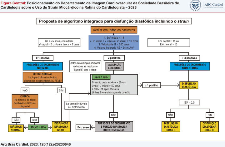
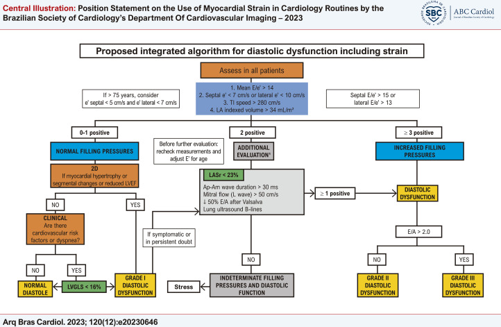
Central Illustration : Position Statement on the Use of Myocardial Strain in Cardiology Routines by the Brazilian Society of Cardiology's Department Of Cardiovascular Imaging - 2023 Proposal for including strain in the integrated diastolic function assessment algorithm, adapted from Nagueh et al.67 Am: mitral A-wave duration; Ap: reverse pulmonary A-wave duration; DD: diastolic dysfunction; LA: left atrium; LASr: LA strain reserve; LVGLS: left ventricular global longitudinal strain; TI: tricuspid insufficiency. Confirm concentric remodeling with LVGLS. In LVEF, mitral E wave deceleration time < 160 ms and pulmonary S-wave < D-wave are also parameters of increased filling pressure. This algorithm does not apply to patients with atrial fibrillation (AF), mitral annulus calcification, > mild mitral valve disease, left bundle branch block, paced rhythm, prosthetic valves, or severe primary pulmonary hypertension.

Figura Central. : Posicionamento do Departamento de Imagem Cardiovascular da Sociedade Brasileira de Cardiologia sobre o Uso do Strain Miocárdico na Rotina do Cardiologista – 2023

Figura 1.1. – A deformação miocárdica pormenorizada em diferentes eixos. A) A deformação básica pode ser aferida nos sentidos longitudinal, circunferencial e radial.4 A partir da interação de dois desses vetores-força, há o surgimento de um terceiro vetor resultante. B) Shear-strain radial-circunferencial. C) Shear-strain longitudinal-circunferencial (que equivale a torção ventricular/torsion). D) Shear-strain radial-circunferencial.

Figura 1.2. – Medidas de pico extraídas das curvas de deformação. A) O strain pico sistólico, o strain pico e strain do final da sístole (ES) coincidem no momento do fechamento da valva aórtica (AVC). B) O strain de pico sistólico e o strain de pico coincidem, porém ambos acontecem imediatamente antes do fechamento da valva aórtica (pequena barra vermelha), produzindo uma discreta dissociação entre aqueles e o strain do final da sístole (ES). C) O strain de pico sistólico e o strain do final da sístole (ES) coincidem (ambos apresentando valores absolutos reduzidos), porém o strain de pico ocorre após o fechamento da valva aórtica (fenômeno de encurtamento pós-sistólico).

Figura 1.3. – Passo a passo para obtenção do strain longitudinal global. Inicialmente, adquirem-se imagens em 3, 4 e 2 câmaras, com eletrocardiograma de boa qualidade e com frame rate adequado (entre 40 e 80 quadros por segundo) (Imagem A, ovoide azul). Marca-se o fechamento da valva aórtica (AVC) a partir do traçado de Doppler pulsátil ou contínuo (Imagem B). Em seguida, faz-se a marcação de três pontos (dois na base e um no ápice), nas três imagens adquiridas, observando se o software faz um de rastreio adequado das imagens 2D (Imagens C e D). Finalmente, obtemos as curvas (Imagem E), o bull’s eye (Imagem F) e o valor obtido do strain longitudinal global. Adaptado de Tressino et al.4

Figura 2.1. – Padrões de SLG com aspecto de poupar a ponta em diferentes cardiopatias. 1: Cardiotoxicidade por antracíclico; 2: Miocárdio não compactado; 3: Hipotireoidismo; 4: Amiloidose por transtirretina.

Figura 2.2. – Padrão de strain avaliado no mapa polar: A: Padrão típico de amiloidose (poupa o ápex); B: Padrão típico de cardiomiopatia hipertrófica com predomínio apical (strain reduzido predominante no ápex, em que a hipertrofia foi evidenciada como mais acentuada no estudo bidimensional).

Figura 3.1. – Exemplo de cardiotoxicidade subclínica em paciente com câncer de mama. Análise da FEVE pelo método de Simpson e do SLG com imagem do bull’s eye. Em A e B, avaliação pré-quimioterapia; em B e C, avaliação após dose cumulativa de 240 mg/m2 de doxorrubicina. Não houve queda expressiva da FEVE, entretanto, foi observada queda relativa de 22% no SLG. FEVE: fração de ejeção do ventrículo esquerdo; SLG: strain longitudinal global.

Figura 3.2. – Algoritmo de avaliação do paciente oncológico durante o tratamento quimioterápico, baseado na FEVE e SLG. CV: cardiovascular; ECA: enzima conversora da angiotensina; FEVE: fração de ejeção do ventrículo esquerdo; QT: quimioterapia; SLG: strain longitudinal global.

Figura 3.3. – Monitoramento ecocardiográfico durante o tratamento com antraciclinas. FEVE: fração de ejeção do ventrículo esquerdo; SLG: strain global longitudinal.

Figura 3.4. – Monitoramento ecocardiográfico durante o tratamento com trastuzumabe. FEVE: fração de ejeção do ventrículo esquerdo; SLG: strain global longitudinal.

Figura 5.1. – A) exemplo de strain longitudinal global (SLG) normal do ventrículo esquerdo. Observam-se as deflexões negativas das curvas, que se apresentam relativamente homogêneas nas três incidências. Abaixo e à direita, a representação paramétrica em bull’s eye, com todos os campos em vermelho mais intenso, significando uma boa deformação global. B) exemplo de strain em um indivíduo portador de cardiomiopatia dilatada de etiologia chagásica. É possível observar a redução de amplitude das curvas, que aqui se apresentam também muito heterogêneas. As curvas de strain septal e na parede inferior têm deflexão positiva, ou seja, indicando distensão ou discinesia, o que está bem demonstrado mapa de bull´s eye em azul (setas amarelas), além do vermelho menos intenso, representando baixos valores de strain (SLG = -5,6%).

Figura 5.2. – A. Imagem bidimensional demonstrando hipertrofia septal assimétrica não obstrutiva, com septo interventricular medindo 23 mm e parede posterior de 11 mm. B. Strain longitudinal global normal do ventrículo esquerdo (20%), com representação paramétrica em bull’s eye, demonstrando segmentos com boa deformação miocárdica em vermelho mais intenso e menores valores de deformação nos segmentos septais, representados na cor rosa (8%). C. Incidência de 4 câmaras, com pior deformação miocárdica nos segmentos médio e basal ínfero-septal. D. Observa-se a redução de amplitude das curvas que representam os segmentos septais, também demonstrado mapa de bull´s eye em rosa, representando valores menores de strain (8%).

Figura 6.1. – Dois pacientes com estenose aórtica grave clássica, de alto fluxo, com fração de ejeção (FE) do ventrículo esquerdo normal, mas valores bastante distintos de strain longitudinal global (SLG). (A) Gradiente transvalvar aórtico médio = 61 mmHg, com FE e SLG normais. (B) Gradiente transvalvar aórtico médio = 88 mmHg, com FE normal e SLG diminuído.

Figura 7.1. – Strain 2D visualizado através do bull’s eye demonstra alteração de deformidade na região apical do ventrículo esquerdo, com valores dos segmentos envolvidos reduzidos, compatível com lesão de artéria descendente anterior.

Figura 8.1. – Strain 2D longitudinal do ventrículo esquerdo em paciente com amiloidose cardíaca ATTR, demonstrando padrão de preservação relativa apical ou apical sparing, com maior acometimento da deformação segmentar em segmentos médios e basais, com maior deformação nos segmentos apicais.

Figura 8.2. – Strain 2D longitudinal do ventrículo direito em paciente com amiloidose cardíaca ATTR, demonstrando redução do valor absoluto global (SLGVD = 9,9%) e redução absoluta do strain médio de parede livre (11,4%), com maior acometimento da deformação segmentar em segmentos médios e basais, com maior deformação nos segmentos apicais.

Figura 8.3. – Amiloidose ATTR. Strain 2D radial do ventrículo esquerdo (VE) na porção basal, demonstrando importante redução dos valores absolutos em todos os segmentos (A). Há também alteração do strain circunferencial, resultando em significativa redução do twist (4o) e torção do VE (B).

Figura 8.4. – Amiloidose AL. Strain bidimensional do átrio esquerdo (AE), com análise das janelas apical 4 câmaras e apical 2 câmaras demonstrando importante redução do valor do strain de AE biplanar (strain reservatório = 4%).

Figura 8.5. – Amiloidose ATTR. Na janela apical ao bidimensional (A), podemos observar a presença de grande massa móvel no interior do átrio direito em paciente com ritmo sinusal. Ao ecocardiograma transesofágico tridimensional (B), em imagem renderizada, observa-se a grande massa aderida ao apêndice atrial direito, correspondendo a trombo. IAS: septo interatrial; SVC: veia cava superior; TV: valva tricúspide.

Figura 8.6. – Strain global longitudinal, em paciente com doença de Fabry, mostrando, no bull’s eye, os valores mais reduzidos nas porções basais da parede ínfero-lateral do ventrículo esquerdo.

Figura 9.1. – Exemplos de mapa polar do strain longitudinal global (SLG) com as curvas do strain de pico sistólico obtidas em 4C, 2C e 3C. (A) Paciente saudável não hipertenso com SLG preservado; (B) Paciente hipertenso sem hipertrofia ventricular esquerda (HVE) com SLG no limite inferior da normalidade com alteração regional da deformação miocárdica em septo basal; (C) Paciente hipertenso com HVE com SLG reduzido e com maior alteração da deformação miocárdica nos segmentos basais e médios do que nos apicais.

Figura 13.1. – Protocolo de imagem para medir a deformação do ventrículo direito (VD) por meio da ecocardiografia speckle tracking na projeção apical 4 câmaras. A) Janela apical 4 câmaras (forma de aquisição inadequada); B) Janela apical 4 câmaras focada no VD (forma de aquisição adequada). VD4CDL: strain global longitudinal do ventrículo direito; VDPLDL: strain de parede livre do ventrículo direito.

Figura 13.2. – Exemplo de strain de ventrículo direito em paciente com hipertensão pulmonar primária de longa data. Software Tomtec. VD4CDL: strain global longitudinal do ventrículo direito; VDPLDL: strain de parede livre do ventrículo direito.

Figura 13.3. – Exemplo de strain de ventrículo direito em paciente em uso de dispositivo de assistência ventricular. Software Echopac GE. SLG: strain de parede livre do ventrículo direito.

Figura 13.4. – Exemplo de strain de ventrículo direito em paciente transplantado cardíaco. Software Tomtec. RV4CDL: strain global longitudinal do ventrículo direito; RVFWSL: strain de parede livre do ventrículo direito.

Figura 14.1. – Mecanismos envolvidos na disfunção atrial esquerda avaliada pelo strain.

Figura 15.1. – Direção da rotação das fibras subendocárdicas (A); direção da rotação das fibras subepicárdicas (B); e rotação resultante geral do ventrículo esquerdo com a contração simultânea das fibras (C). Adaptado de Stöhr et al.384

Figura 15.2. – Planos de obtenção das imagens para medida da rotação basal e apical. Imagens cedidas pelo Dr. Marcio Lima.

Figura 15.3. – Registro das rotações horária (abaixo da linha de base) e anti-horária (acima da linha de base). Imagens cedidas pelo Dr. Marcio Lima.

Figura 16.1. – Imagem de strain radial com curvas dos segmentos médios das paredes anterosseptal e inferolateral. O intervalo acima de 130 ms correlaciona-se com uma maior taxa de resposta à terapia de ressincronização cardíaca; nesse caso, 340 ms.

Figura 16.2. – Imagem do strain longitudinal com curvas dos segmentos basais inferosseptal (amarela) e anterolateral (vermelha) com padrão de bloqueio de ramo esquerdo típico: 1) oposição do pico das curvas septal (negativa) e lateral (positiva), inicialmente; 2) pico de deformação negativa do septo em até 70% do tempo de ejeção, com o encurtamento sendo interrompido durante a sístole, isto é, antes do fechamento da valva aórtica (AVC), resultando em estiramento sistólico; 3) pico de deformação negativa de parede lateral após o fechamento da valva aórtica.

Figura 16.3. – Mapas polares comparativos pré- e pós-procedimento do strain longitudinal (A), do myocardial work (B), myocardial efficiency (C) em paciente submetido a terapia de ressincronização com sucesso.

Figura 17.1. – Alça pressão vs. deformação do ventrículo esquerdo. Em vermelho: alça pressão vs. deformação global do ventrículo esquerdo. Em verde: alça pressão-deformação do segmento basal da parede ínfero-lateral. LVP: pressão do ventrículo esquerdo estimada pela pressão arterial sistólica; AVO: abertura da válvula aórtica; AVC: fechamento da válvula aórtica; MVO: abertura da válvula mitral; MVC: fechamento da válvula mitral.

Figura 17.2. – Após a realização da análise de strain bidimensional longitudinal do ventrículo esquerdo pelo método AFI (automated functional imaging), tendo processado as três janelas apicais, o software oferece a opção de cálculo do trabalho miocárdico (myocardial work) – seta.

Figura 17.3. – Tela inicial de cálculo do trabalho miocárdico. Podemos inserir manualmente, nessa etapa, o valor da pressão arterial não invasiva aferida (seta) e reavaliar ou realizar a marcação de eventos cardíacos, como a abertura e fechamento das valvas mitral e aórtica (setas).

Figura 17.4. – Marcação de eventos cardíacos com o uso do Doppler espectral. Em A, observamos a marcação de abertura (MVO) e o fechamento da valva mitral (MVC) através do influxo mitral. Em B, observamos a marcação de abertura (AVO) e o fechamento da valva aórtica (AVC) através do fluxo da via de saída do ventrículo esquerdo.

Figura 17.5. – A marcação de eventos cardíacos também pode ser realizada na própria tela de cálculo do trabalho miocárdico (myocardial work), modificando quadro a quadro (“frame”) a imagem do apical 3 câmaras, selecionando o momento exato de cada evento, clicando nos campos à direita (setas).

Figura 17.6. – Após a aprovação dos dados obtidos, a marcação adequada de eventos e o preenchimento de pressão não invasiva, o software dispõe os valores de strain longitudinal global e por segmento à esquerda (setas brancas) e os mapas polares com valores de índice de trabalho miocárdico (A – seta amarela) e de eficiência de trabalho miocárdico (B – seta azul).

Figura 17.7. – Quando selecionamos a tecla “advanced”, são geradas as análises por curvas e gráficos, onde é possível observar as alças de pressão do ventrículo esquerdo (left ventricular pressure, LVP) vs. strain ao longo do ciclo cardíaco (seta amarela), além de um gráfico de barras que demonstra a participação do trabalho miocárdico construtivo e do trabalho miocárdico desperdiçado (seta azul).

Figura 17.8. – Casos 1 e 2 com morfologias bem semelhantes de bloqueio de ramo esquerdo.

Figura 17.9. – Caso 1 não apresenta alteração na mecânica miocárdica visualizado pela linha verde em que o trabalho miocárdico na alça pressão-strain é semelhante ao valor global em vermelho. Já no Caso 2, o “verdadeiro” bloqueio de ramo esquerdo, note que na mesma porção septal a curva em verde adquire um formato típico de 8.

Figura 19.1. – Análise do strain longitudinal global pelo método de feature tracking em paciente com hipertensão pulmonar (acima) e sem hipertensão pulmonar (abaixo). O paciente com hipertensão pulmonar apresentou strain de 4,26% e o sem hipertensão pulmonar de 26,46%.

Central Illustration. : Position Statement on the Use of Myocardial Strain in Cardiology Routines by the Brazilian Society of Cardiology’s Department Of Cardiovascular Imaging – 2023

Figure 1.1. – Myocardial strain in different axes. A) Strain can be measured in the longitudinal, circumferential, and radial directions.4 A third vector results from the interaction of 2 of these force-vectors. B) Radial-circumferential shear strain. C) Longitudinal-circumferential shear strain (ie, ventricular twist/torsion). D) Radial-circumferential shear strain.

Figure 1.2. – Peak measurements derived from strain curves A) Peak systolic strain, peak strain, and end-systolic (ES) strain coincide upon aortic valve closure (AVC). B) Peak systolic strain and peak strain coincide, although both occur immediately before AVC (red bar), resulting in slight dissociation between these and ES strain. C) Peak and end-systolic strain coincide (both with lower absolute values), although peak strain occurs after AVC (post-systolic shortening phenomenon).

Figure 1.3. – Step by step to obtain the global longitudinal strain. Initially, images are acquired in 3, 4 and 2 chambers, with good quality EKG. Images must be acquired at an adequate frame rate (40-80 frames per second) (A: blue ovoid). Aortic valve closure (AVC) is marked using pulsed or continuous Doppler tracking (B). Three points (2 at the base and 1 at the apex) are then marked on the 3 acquired images, determining whether the software adequately tracked the 2D images (C and D). Finally, the curves (E), bull’s eye map (F), and global longitudinal strain values are obtained. Adapted from Tressino et al.4

Figure 2.1. – Global longitudinal strain with apical sparing patterns in different heart diseases. 1: Anthracycline cardiotoxicity; 2: Non-compacted myocardium; 3: Hypothyroidism; 4: Transthyretin amyloidosis.

Figure 2.2. – Strain pattern in polar mapping: A: Typical amyloidosis pattern (apical sparing); B: Typical hypertrophic cardiomyopathy pattern with apical predominance (lower strain predominates in the apex, where hypertrophy was more pronounced in 2D assessment).

Figure 3.1. – Example of subclinical cardiotoxicity in a patient with breast cancer. Analysis of LVEF through Simpson’s method and GLS with bull’s eye mapping. A and B: pre-chemotherapy evaluation; B and C: evaluation after a cumulative dose of 240 mg/m2 of doxorubicin. Although there was no significant reduction in LVEF, there was a 22% relative decrease in GLS. LVEF: left ventricular ejection fraction; GLS: global longitudinal strain.

Figure 3.2. – Algorithm for evaluating cancer patients during chemotherapy treatment, based on LVEF and GLS. ACE: angiotensin-converting enzyme; CV: cardiovascular; CT: chemotherapy Echo: echocardiography; GLS: global longitudinal strain; HF: heart failure; LVEF: left ventricular ejection fraction.

Figure 3.3. – Echocardiographic monitoring during anthracycline therapy. Echo: echocardiography; GLS: global longitudinal strain; LVEF: left ventricular ejection fraction.

Figure 3.4. – Echocardiographic monitoring during trastuzumab therapy. Echo: echocardiography. GLS: global longitudinal strain; LVEF: left ventricular ejection fraction.

Figure 5.1. – A) Example of normal left ventricle global longitudinal strain. Note the negative deflections of the curves, which are relatively homogeneous in the 3 views. In the lower right is the parametric bull’s eye mapping, with all fields in more intense red, indicating good global strain; B) Example of strain in an individual with dilated cardiomyopathy due to Chagas disease. Note the reduced amplitude of the curves, which are also very heterogeneous. The septal and inferior wall strain curves have a positive deflection, ie, indicating distension or dyskinesia, which in the bull’s eye map appears blue (yellow arrows), in addition to pink areas, which indicate low strain values (GLS = -5.6%).

Figure 5.2. – A) Two-dimensional image demonstrating non-obstructive asymmetric septal hypertrophy, with an interventricular septum measuring 23 mm and a posterior wall measuring 11 mm; B) normal global longitudinal strain (GLS) of the LV (20%), with parametric bull’s eye mapping segments with good myocardial strain are darker red, while pink indicates lower strain values in the septal segments (8%); C) 4-chamber view, with lower myocardial strain in the middle and basal inferoseptal segments; D) note the reduced amplitude of the curves representing septal segments, also shown in pink in the bull’s eye map, representing lower strain values (8%).

Figure 6.1. – Two patients with classic severe high-flow aortic valve stenosis with normal left ventricular ejection fraction (LVEF) but very different global longitudinal strain (GLS) values. (A) Mean aortic transvalve gradient = 61 mm Hg, with normal EF and GLS. (B) Mean aortic transvalve gradient = 88 mm Hg, with normal EF and reduced GLS.

Figure 7.1. – Two-dimensional bull’s eye mapping showing strain in the apical region of the left ventricle; the reduced segmental values are compatible with injury in the anterior descending artery.

Figure 8.1. – Longitudinal 2D strain of the left ventricle in a patient with cardiac transthyretin amyloidosis, showing relative apical preservation (apical sparing pattern), with lower strain in the middle and basal segments and higher strain in the apical segments.

Figure 8.2. – Longitudinal 2D strain assessment in the right ventricle of a patient with cardiac transthyretin amyloidosis, showing a lower absolute global value (RVGLS = 9.9%) and an absolute reduction in mean free wall strain (FWS) (11.4%), with lower values in middle and basal segments and higher values in apical segments. TAPSE: tricuspid annular plane systolic excursion.

Figure 8.3. – Transthyretin amyloidosis. Significantly lower absolute left ventricular (LV) radial strain values in all basal segments in 2D assessment (A). There is also a change in circumferential strain, resulting in significantly reduced “twist” (4º) and LV torsion (B).

Figure 8.4. – Immunoglobulin light chain amyloidosis. Two-dimensional left atrial (LA) strain, with 4-chamber and 2-chamber apical windows, showing an important reduction in LA strain (reservoir strain = 4%).

Figure 8.5. – Transthyretin amyloidosis. The 2D apical window shows: (A) a large mobile mass inside the right atrium in a patient with sinus rhythm; (B) a 3D-rendered transesophageal echocardiography image showing a large mass (thrombus) adhered to the right atrial appendage. IAS: interatrial septum; SVC: superior vena cava; TV: tricuspid valve.

Figure 8.6. – Global longitudinal strain in a patient with Fabry disease: bull’s eye map shows the lowest values in the in the basal portions of the left ventricle inferolateral wall. AVC: aortic valve closure.

Figure 9.1. – Examples of global longitudinal strain polar mapping with peak systolic strain curves obtained in 4, 2 and 3 chambers. (A) healthy non-hypertensive patient with preserved GLS; (B) hypertensive patient without LV hypertrophy whose GLS is at the lower limit of normality (note altered myocardial strain in the basal septum); (C) hypertensive patient with LV hypertrophy and reduced GLS (note greater change in myocardial strain in basal and middle segments than apical segments).

Figure 13.1. – Imaging protocol for right ventricular (RV) strain measurement through speckle tracking echocardiography in an apical 4-chamber view: A) apical 4-chamber window (inappropriate acquisition method); B) apical 4-chamber window focused on the RV (adequate acquisition method). RVFWS: RV free wall strain; RVGLS: RV global longitudinal strain.

Figure 13.2. – Example of right ventricular (RV) strain in a patient with primary pulmonary hypertension. TomTec software. RVFWS: RV free wall strain; RVGLS: RV global longitudinal strain.

Figure 13.3. – Example of right ventricular strain in a patient using a ventricular assist device. GE EchoPAC software. AVC: aortic valve closure; GLS: global longitudinal strain.

Figure 13.4. – Example of right ventricular strain in a heart transplant patient. TomTec Software. RVFWS: right ventricular free wall strain; RV4CS: right ventricular global longitudinal strain.

Figure 14.1. – Strain assessment of mechanisms involved in left atrial dysfunction.

Figure 15.1. – Rotation direction of subendocardial fibers: (A) subepicardial fibers (B) overall LV rotation with (C) simultaneous contraction of the fibers. Adapted from Stöhr et al.384

Figure 15.2. – Image acquisition plan for basal and apical rotation measurement (Images courtesy of Dr. Marcio Lima).

Figure 15.3. – Clockwise (below baseline) and counterclockwise (above baseline) rotation (Images courtesy of Dr. Marcio Lima).

Figure 16.1. – Radial strain image showing curves for the middle segments of the anteroseptal and inferolateral walls. The interval > 130 ms correlates with a higher CRT response rate, in this case 340 ms.

Figure 16.2. – Longitudinal strain image with inferoseptal (yellow) and anterolateral (red) basal segment curves with typical left bundle branch block pattern: 1) initial opposition of the peak of the septal (negative) and lateral (positive) curves; 2) negative septal strain peak in ≤ 70% of the ejection time, with shortening interrupted during systole, ie, prior to aortic valve closure (AVC) resulting in systolic stretching; 3) negative strain peak in the lateral wall after AVC.

Figure 16.3. – Pre- and post-procedure polar maps of (A) longitudinal strain, (B) myocardial work, and (C) myocardial efficiency in a patient who underwent successful resynchronization therapy.

Figure 17.1. – Left ventricular pressure-strain loop. Red: global pressure-strain loop. Green: pressure-strain loop for the basal segment of the inferolateral wall. AVC: aortic valve closure; AVO: aortic valve opening; IVCT: isovolumetric contraction time; IVRT: isovolumetric relaxation time LVP: left ventricular pressure estimated by systolic blood pressure; MVC: mitral valve closure; MVO: mitral valve opening.

Figure 17.2. – After assessing 2D LV longitudinal strain with the automated functional imaging method and processing the 3 apical windows, the software offers to calculate myocardial work (yellow arrow).

Figure 17.3. – Initial screen of myocardial work calculation. In this step, non-invasively measured blood pressure values can be inserted (bottom arrow), and cardiac events, such as the opening and closing of the mitral and aortic valves can be reassessed or marked (top arrow).

Figure 17.4. – Marking cardiac events through spectral Doppler: A) marking mitral valve opening (MVO) and mitral valve closing (MVC) according to mitral inflow; B) marking aortic valve opening (AVO) and aortic valve closing (AVC) through LV outflow.

Figure 17.5. – Cardiac events can also be marked on the myocardial work calculation screen, modifying apical 3-chamber images frame by frame and selecting the exact moment of each event in the right sidebar menu (arrows).

Figure 17.6. – After approval of the obtained data, appropriately marking events and pressure filling, the software displays the global and segmental longitudinal strain values on the left (white arrows) and polar maps with myocardial work index values (A: yellow arrow) and myocardial work efficiency (B: blue arrow).

Figure 17.7. – Selecting the “advanced” key shows analyses by curves and graphs, showing the LV pressure-strain loops throughout the cardiac cycle (yellow arrow), in addition to a bar chart showing the proportions of constructive and wasted MW (blue arrow).

Figure 17.8. – Two cases with similar left bundle branch block morphologies.

Figure 17.9. – Case 1 has no changes in myocardial mechanics: myocardial work in the pressure-strain loop (green line) is similar to the global value (red line). In case 2, “true” left bundle branch block; in the same septal portion, the green line assumes a figure-8 shape.

Figure 19.1. – Global longitudinal strain analysis through feature tracking in patients with (above) and without pulmonary hypertension (below). GLS was 4.26% and 26.46% in the patients with and without pulmonary hypertension, respectively.

References

1. Loizou CP, Pattichis CS, D’Hooge J. Handbook of Speckle Filtering and Tracking in Cardiovascular Ultrasound Imaging and Video. London: The Institution of Engineering and Technology; 2018.
1. Sutherland GR, Di Salvo G, Claus P, D’hooge J, Bijnens B. Strain and Strain Rate Imaging: A New Clinical Approach to Quantifying Regional Myocardial Function. J Am Soc Echocardiogr. 2004;17(7):788–802. doi: 10.1016/j.echo.2004.03.027. - DOI - PubMed
1. D’hooge J, Heimdal A, Jamal F, Kukulski T, Bijnens B, Rademakers F, et al. Regional Strain and Strain Rate Measurements by Cardiac Ultrasound: Principles, Implementation and Limitations. Eur J Echocardiogr. 2000;1(3):154–170. doi: 10.1053/euje.2000.0031. - DOI - PubMed
1. Tressino CG, Hortegal RA, Momesso M, Barretto RBM, Le Bihan D. Como eu Faço: Avaliação do Strain do Ventrículo Esquerdo. Arq Bras Cardiol: Imagem Cardiovasc. 2020;33(4):ecom15. doi: 10.47593/2675-312X/20203304ecom15. - DOI
1. Hortegal R, Abensur H. Strain Echocardiography in Patients with Diastolic Dysfunction and Preserved Ejection Fraction: Are We Ready? Arq Bras Cardiol: Imagem Cardiovasc. 2017;30(4):132–139. doi: 10.5935/2318-8219.20170034. - DOI
Publication types