A Modular Implementation to Handle and Benchmark Drift Correction for High-Density Extracellular Recordings

Abstract

High-density neural devices are now offering the possibility to record from neuronal populations in vivo at unprecedented scale. However, the mechanical drifts often observed in these recordings are currently a major issue for "spike sorting," an essential analysis step to identify the activity of single neurons from extracellular signals. Although several strategies have been proposed to compensate for such drifts, the lack of proper benchmarks makes it hard to assess the quality and effectiveness of motion correction. In this paper, we present a benchmark study to precisely and quantitatively evaluate the performance of several state-of-the-art motion correction algorithms introduced in the literature. Using simulated recordings with induced drifts, we dissect the origins of the errors performed while applying a motion correction algorithm as a preprocessing step in the spike sorting pipeline. We show how important it is to properly estimate the positions of the neurons from extracellular traces in order to correctly estimate the probe motion, compare several interpolation procedures, and highlight what are the current limits for motion correction approaches.

Keywords: benchmark; drift; electrophysiology; ground-truth; neuropixel; spike sorting.

Figure 1.

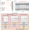
Common pipeline for drift correction algorithms. A, Illustration of the problems raised by neuronal drifts. Two neurons (red and orange) have two distinct waveforms, but after some non-rigid drifts (movements), the templates are changed. B, Illustration of the drift in vivo. A Neuropixels 1.0 probe in the cortex of the mice is moved up and down with an imposed triangular movement of amplitude 50 m (top trace; Steinmetz, 2021; Steinmetz et al., 2021)—p1 dataset. The row shows the depth of all the peaks detected via signal threshold (positional raster plot, see text) as a function of time. When the probe starts moving (red dotted line), so does the depth of the peaks, since neurons are drifting across channels. While the drift here is imposed, spontaneous drifts can happen locally and non-homogeneously over the whole probe (see inside light blue boxes for before and after imposed motion). Panels A and B are adapted from Buccino et al. (2022), with permission. C, Key algorithmic steps for the motion correction pipeline. For each step, the various implementations available in SpikeInterface are listed. The yellow boxes connected with arrows correspond to a Kilosort 2.5/3-like approach (Pachitariu et al., 2023).

Figure 2.

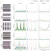
Examples of simulated drift recordings. For each panel, the top shows the layout of the probe with superimposed starting position of each cell (left), the positional raster plot with overlaid GT motion signals (center), and the depth distribution of the 256 neurons. The bottom part displays the firing rate modulation. Here we display 5 out of 12 recordings (the remaining 7 can be found as Extended data Figure on the github repo of the project). A, Rigid ZigZag drift with uniform depth distribution and homogeneous firing rates. B, Rigid ZigZag drift with bimodal depth distribution and homogeneous firing rates. C, Non-rigid ZigZag with uniform depth distribution and modulated firing rates. D, Non-rigid ZigZag with uniform depth distribution and homogeneous firing rates. E, Bumps with uniform depth distribution and homogeneous firing rates.

Figure 3.

Motion estimation performance for different simulation modes. A, Top: distribution of the log errors for all the errors pooled over all motion correction pipelines tested in this paper, as a function of the types of drift (ZigZag, ZigZag (non-rigid), or bumps). Bottom: averaged error over all methods, as a function of the probe depth and the nature of the drift. B, Same as in A, but as a function of the type of the depth distribution (uniform and bimodal) of the neurons. C, Same as in A, but as a function of the firing rate profiles.

Figure 4.

Performance in motion estimation for various drift scenarios. For various situations of the drifts with overlaid GT motion (left column), errors (from left to right) as a function of time (time error), averaged (global error), or as a function of the depths (depth error) and for various motion estimation pipelines. Here we display 5 out of 12 recordings (the remaining 7 can be found in the github repo of the project). A, Zigzag (rigid), bimodal positions, homogeneous rates. B, Zigzag (rigid), bimodal positions, homogeneous rates. C, Zigzag (non-rigid), uniform positions, modulated rates. D, Zigzag (non-rigid), uniform positions, homogeneous rates. E, Bump (non-rigid), uniform positions, homogeneous rates.

Figure 5.

Motion estimation performance for the bumps (non-rigid) drift case. A, Positional raster plot to show the movement of the cells, during the simulated drift. B, The errors with respect to the GT motion vector as a function of the time (time error), averaged over time (global error), or as a function of the depth (depth error) for several motion estimation pipelines. C, Run time of the different pipeline to estimate the motion (see legend below). D, Errors, as a function of depth and time, for all the motion estimation methods considered. The time course of the averaged drift vector is shown at the bottom.

Figure 6.

Quantification of the interpolation methods. A, Positional raster plots with a bumps (non-rigid) drift (uniform/homogeneous) for the static (gray), drifting (red), and interpolated traces via Kriging (green), IDW (orange), or Snap (blue), using the GT motion vector. Note that the probe is cropped here for visibility purposes. B, Top: flattened template (on a subset of channels) for a single neuron in all the conditions (static, drifting, and the three interpolation methods), in units of the median absolute deviation (mad) of the noise on the considered channels. Bottom: STD over time, normalized by the template RMS, of all the individual spikes for this particular neuron, in the same conditions. C, Ratios of waveform STD compared to the static case for all the cells in the recording, in all conditions, and as a function of the depth of the neurons. Right panel displays the overall STD ratio distributions. In this case, an STD ratio above 1 means an increase in waveforms dispersion with respect to the static case (and a decrease for ratios below 1).

Figure 7.

Quantification of the interpolation on sorting accuracy. A, D, G, Accuracy of all units (sorted by accuracy) in the simulated recordings when launching Kilosort 2.5 in various conditions for the Zigzag rigid case (A), the Zigzag (non-rigid case) (D), or the bumps (non-rigid) case (G). All recordings have uniform distributions and homogeneous firing rates. B, E, H, Number of well detected/overmerged/redundant/false positive and bad units found by Kilosort , with various drift correction methods, for the recordings explained in A, D, G. C, F, I, The loss in accuracy for the well-detected neurons (accuracy higher than 0.8—N = 164) between the static case and the one using Mono + Dec estimation, as a function of the depth of the neurons (x axis) and the SNR (y axis).

References

1. Angotzi GN, Boi F, Lecomte A, Miele E, Malerba M, Zucca S, Casile A, Berdondini L (2019) SiNAPS: an implantable active pixel sensor CMOS-probe for simultaneous large-scale neural recordings. Biosens Bioelectron 126:355–364. 10.1016/j.bios.2018.10.032 - DOI - PubMed
1. Berdondini L, Imfeld K, Maccione A, Tedesco M, Neukom S, Koudelka-Hep M, Martinoia S (2009) Active pixel sensor array for high spatio-temporal resolution electrophysiological recordings from single cell to large scale neuronal networks. Lab Chip 9:2644–2651. 10.1039/b907394a - DOI - PubMed
1. Boussard J, Varol E, Dong Lee H, Dethe N, Paninski L (2021) Three-dimensional spike localization and improved motion correction for neuropixels recordings. Adv Neural Inf Process Syst 34:22095–22105.
1. Boussard J, Windolf C, Hurwitz C, Lee HD, Yu H, Winter O, Paninski L (2023) “DARTsort: A Modular Drift Tracking Spike Sorter for High-Density Multi-electrode Probes.” bioRxiv, pp 2023–08.
1. Buccino AP, Einevoll GT (2020) Mearec: a fast and customizable testbench simulator for ground-truth extracellular spiking activity. Neuroinformatics 19:185–204. 10.1007/s12021-020-09467-7 - DOI - PMC - PubMed
LinkOut - more resources