An 8-model ensemble of CMIP6-derived ocean surface wave climate

Abstract

We present a global wind wave climate model ensemble composed of eight spectral wave model simulations forced by 3-hourly surface wind speed and daily sea ice concentration from eight different CMIP6 GCMs. The spectral wave model uses ST6 physics parametrizations and a global three-grid structure for efficient Arctic and Antarctic wave modeling. The ensemble performance is evaluated against a reference global multi-mission satellite altimeter database and the recent ECMWF IFS Cy46r1 ERA5 wave hindcast, ERA5H. For each ensemble member three 30-year slices, one historical, and two future emission scenarios (SSP1-2.6 and SSP5-8.5) are available, and cover two distinct periods: 1985-2014 and 2071-2100. Two models extend to 140 years (1961-2100) of continuous wind wave climate simulations. The present ensemble outperforms a previous CMIP5-forced wind wave climate ensemble, showing improved performance across all ocean regions. This dataset is a valuable resource for future wind wave climate research and can find practical applications in offshore and coastal engineering projects, providing crucial insights into the uncertainties connected to wind wave climate future projections.

Fig. 1

Gantt chart (time duration) of the WW3 8-model wave climate ensemble. In orange, the CMIP historical runs, in light blue the SSP1-2.6 mid-emission scenario, and in blue the SSP5-8.5 high-emission scenario. Note that, the WW3/ACM2 and the WW3/EC3 models were also run for 140 years of continuous wave climate projections. The rest of the models composing the ensemble are run for the CMIP historical 1985–2014 and the SSP1-2.6 and SSP5-8.5 2071–2100 30-year time slices.

Fig. 2

Multi-Model Ensemble (MME) spatial distribution performance against satellite altimeter (SAT) and ERA5H hindcast. The 1985–2014 (a) U₁₀ and (b) H_s MME average climatology. (c,d) The MME 1992–2014 U₁₀ absolute and relative error in comparison with the SAT climatology. (e,f) Same as (c,d) but for H_s. (g,h) The MME 1985–2014 H_s absolute and relative error in comparison to ERA5H.

Fig. 3

The 1992–2014 (a) H_s and (b) $H_{\mathrm{s}}^{p90}$, mean and 90th percentile significant wave height climatology in relation to the 2° × 2° satellite altimeter (SAT) (represented by a black star) for each WW3/GCM model ensemble member. The ERA5H performance in relation to the SAT dataset over the same period is marked with a black square. The x and y axis represent the standard deviation normalized by the reference SAT standard deviation (σ_SAT). The SAT statistic is placed at the x-axis unit as a reference point. The radial position on the graph represents the Pearson correlation coefficient calculated for each instance of WW3/GCM and ERA5H models against the SAT dataset. The concentric grey circles centered in the black star (x-axis unit) illustrate the Root Mean Square Error (RMSE) values in comparison to SAT.

Fig. 4

The 1985–2014 RMSE portrait diagram of relative seasonal (DJF, MAM, JJA, and SON) error metrics for each WW3/GCM ensemble member in relation to ERA5H. Each WW3/GCM performance is plotted relative to the median of the ensemble (S_i in Eq. 1). Each row is a WW3/GCM ensemble member, and each column a different integral parameter output, namely: the average and the 90th percentile significant wave height, H_s and $H_{\mathrm{s}}^{p90}$, the mean second-order spectral wave period, T_{m, 02}, the mean wave direction, θ, and the wave energy flux, C_gE. The models with a smaller (larger) RMSE than the ensemble median RMSE are shown in blue (red). Overall, the WW3/ACM2 is the best performing model and the WW3/MRI is the ensemble member with the poorest performance.

Fig. 5

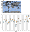
The present 1985–2014 CMIP6 and the 1979–2004 CMIP5 wave climate ensembles performance in relation to ERA5H. (a) Alves reference ocean climatic regions: Tropical North Indian Ocean (TNIO), Extra-Tropical South Atlantic (ETSA), Tropical South Atlantic Ocean (TSAO), Tropical North Atlantic Ocean (TNAO), Extra-Tropical North Atlantic (ETNA), Extra-Tropical South Pacific (ETSP), Tropical Eastern South Pacific (TESP), Tropical Western South Pacific (TWSP), Tropical Eastern North Pacific (TENP), Tropical Western North Pacific (TWNP), Extra-Tropical North Pacific (ETNP), Extra-Tropical South Indian (ETSI), and Tropical South Indian Ocean (TSIO). (b) The M-score metrics by ocean climatic regions for the CMIP5 (light blue) and the CMIP6 (orange) ensemble members. Each WW3/GCM M-Score is computed by averaging the M-score of three integral parameter outputs: H_s, T_{m, 02} (T_{m, 01} for CMIP5), and θ. The results are clustered into a box-plot that shows the median ensemble M-score, the Inter-Quartile Range and the minimum and maximum M-score values of each ensemble member.

Fig. 6

Potential applications of the present CMIP6 wave climate model ensemble. Global future projected wind-wave climate changes. The Δ in each panel refers to the difference between the end of the 21^st century (2071–2100) and the historical (1985–2014) climatology. The figure shows the SSP1-2.6 (left column) and the SSP5-8.5 (right column) future projected MME percentage changes of: (a) the significant wave height, $\mathrm{\Delta }{\overline{H}}_{\mathrm{s}}$, (b) the mean second-order spectral wave period, $\mathrm{\Delta }{\overline{T}}_{\mathrm{m,02}}$, and (c) the mean wave direction, $\mathrm{\Delta }\overline{\theta }$. A ‘model democracy’ approach was followed to compute the MME average statistics where each model is equally weighted. The hatching in (a,b) defines where the $\mathrm{\Delta }{\overline{H}}_{\mathrm{s}}$ and $\mathrm{\Delta }{\overline{T}}_{\mathrm{m,02}}$ changes are statistically significant. The change is defined statistical significant if it surpasses the ensemble average SSP1-2.6 and SSP5-8.5 projections inter-annual variability (Figures S5b,c, S6b,c). The arrows in (c) show the 2071–2100 future projected average mean wave directions.

References

1. Lopatoukhin, L. et al. Estimation of extreme wind wave heights. Tech. Rep., WMO (2000).
1. Lowe, J. A. et al. Past and future changes in extreme sea levels and waves (Blackwell, 2010).
1. Young IR, Ribal A. Multiplatform evaluation of global trends in wind speed and wave height. Science. 2019;364:548–552. doi: 10.1126/science.aav9527. - DOI - PubMed
1. Oppenheimer M, et al. Sea level rise and implications for low lying islands, coasts and communities. 2019 doi: 10.1017/9781009157964.006. - DOI
1. Lincke D, Hinkel J, Mengel M, Nicholls RJ. Understanding the drivers of coastal flood exposure and risk from 1860 to 2100. Earth’s Future. 2022;10:e2021EF002584. doi: 10.1029/2021EF002584. - DOI