The Emergence of the Normal Distribution in Deterministic Chaotic Maps

Abstract

The central limit theorem states that, in the limits of a large number of terms, an appropriately scaled sum of independent random variables yields another random variable whose probability distribution tends to attain a stable distribution. The condition of independence, however, only holds in real systems as an approximation. To extend the theorem to more general situations, previous studies have derived a version of the central limit theorem that also holds for variables that are not independent. Here, we present numerical results that characterize how convergence is attained when the variables being summed are deterministically related to one another through the recurrent application of an ergodic mapping. In all the explored cases, the convergence to the limit distribution is slower than for random sampling. Yet, the speed at which convergence is attained varies substantially from system to system, and these variations imply differences in the way information about the deterministic nature of the dynamics is progressively lost as the number of summands increases. Some of the identified factors in shaping the convergence process are the strength of mixing induced by the mapping and the shape of the marginal distribution of each variable, most particularly, the presence of divergences or fat tails.

Keywords: central limit theorem; deterministic systems; stable distributions.

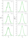
Figure 1

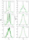
Left, dark line: Numerical results for the distribution ${\rho }_{s_N}$ of the sums $s_N$ defined in Equation (3), in the case the Bernoulli (10) map with $m=2$, for three small values of N. The light curve is the Gaussian expected for $N\to \infty$, and the dashed curve is a Gaussian with the same variance as predicted for ${\rho }_{s_N}$. Right, dark curve: The distribution ${\rho }_{s_N}^{\mathrm{random}}$ for sums of N values of x randomly sampled from ${\rho }_x\left(x\right)$ is a normalized version of the Irwin–Hall distribution [15,16], which can be obtained analytically through the successive self-convolution of ${\rho }_x$. The light curve is the Gaussian expected for $N\to \infty$. Note the different scales on the left and right columns.

Figure 2

Main panel: The Kullback–Leibler divergences $D_G$, $D_{G_N}$, and $D_{\mathrm{random}}$, defined in the text, as functions of the number of terms in the sums $s_N$ of Equation (3), for the Bernoulli map (10) with $m=2$. The straight lines in this log–log plot have a slope $-2$. The inset shows, as dots, numerical results for the variance ${\sigma }_{s_N}^2$ over the distribution ${\rho }_{s_N}\left(s_N\right)$. The dashed line joins the analytical values predicted from Equation (12).

Figure 3

The Kullback–Leibler divergence $D_G$ for the Bernoulli map (10) with various values of m, and $D_{\mathrm{random}}$ (which is the same for all m). The straight lines have slope $-2$.

Figure 4

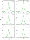
As in Figure 1 for the logistic map of Equation (16) in the regime of full chaos, $\lambda =4$. The distributions ${\rho }_{s_N}^{\mathrm{random}}$, dark lines on the right column, have now been obtained numerically. Note the different scales in different panels.

Figure 5

The Kullback–Leibler divergence $D_G$ for the logistic map of Equation (16) in the regime of full chaos, $\lambda =4$, and $D_{\mathrm{random}}$, as a functions of N. In this case, $D_{G_N}$ coincides with $D_G$. The full and dashed straight lines have slopes $-2$ and $-1$, respectively.

Figure 6

Left: 900 successive iterations of the logistic map, Equation (16), in the intermittent regime, $\lambda =3.828$. The arrows at $t=300$ and 500 point at “turbulent” and period-3 “laminar” intervals, respectively. Right: The correlation $c_k=\overline{[x\left(t\right)-\overline{x}][x(t+k)-\overline{x}]}$ as a function of k in the same intermittent regime, calculated numerically from sequences of ${10}^7$ iterations of $x\left(t\right)$. Symbols are connected by lines to facilitate visualization.

Figure 7

The Kullback–Leibler divergences $D_G$ for the logistic map (16) in the intermittent regime, $\lambda =3.828$, and $D_{\mathrm{random}}$, as functions of N. For the former, triangles correspond to values of N which are multiples of 3. The slope of the dashed straight line is $-1$. Inset: Numerical results for the variance ${\sigma }_{s_N}^2$ of the sums $s_N$, as a function of N. The arrow to the right indicates the variance obtained for large N. Symbols are connected by dashed lines to facilitate visualization.

Figure 8

As in Figure 4, for the sums of Equation (18) with $x\left(t\right)$ obtained from map (20). Note that the scales are the same in all plots.

Figure 9

The Kullback–Leibler divergences $D_C$ and $D_{\mathrm{random}}$ for the distributions of the sums of Equation (18), with the values of x obtained from the map (20) and the distribution of Equation (22), respectively. The full straight line has slope $-1$, and the dashed line, with slope $-0.68$, is a linear fitting of $D_C$ for $N\ge 2$.

References

1. Lévy P. Theorie de L’addition des Variables Aleatoires. Gauthier-Villars; Paris, France: 1937.
1. Gnedenko B.V., Kolmogorov A.N. Limit Distributions for Sums of Independent Random Variables. Addison-Wesley; Cambridge, MA, USA: 1954.
1. Uchaikin V.V., Zolotarev V.M. Chance and Stability: Stable Distributions and Their Applications. Walter de Gruyter; Boston, MA, USA: 2011.
1. Araujo A., Giné E. The Central Limit Theorem for Real and Banach Valued Random Variables. Wiley; New York, NY, USA: 1980.
1. Billingsley P. Probability and Measure. Wiley; New York, NY, USA: 1995.
LinkOut - more resources