Stable fixed points of combinatorial threshold-linear networks

Abstract

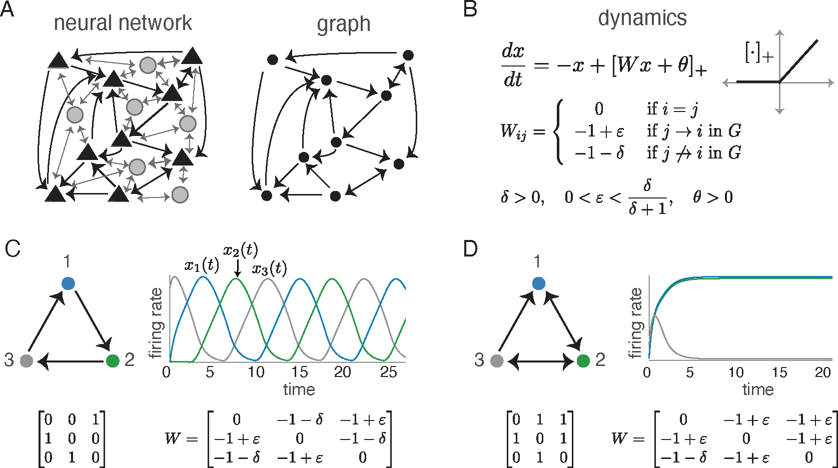
Combinatorial threshold-linear networks (CTLNs) are a special class of recurrent neural networks whose dynamics are tightly controlled by an underlying directed graph. Recurrent networks have long been used as models for associative memory and pattern completion, with stable fixed points playing the role of stored memory patterns in the network. In prior work, we showed that target-free cliques of the graph correspond to stable fixed points of the dynamics, and we conjectured that these are the only stable fixed points possible [1, 2]. In this paper, we prove that the conjecture holds in a variety of special cases, including for networks with very strong inhibition and graphs of size $n\le 4$. We also provide further evi-dence for the conjecture by showing that sparse graphs and graphs that are nearly cliques can never support stable fixed points. Finally, we translate some results from extremal com-binatorics to obtain an upper bound on the number of stable fixed points of CTLNs in cases where the conjecture holds.

Keywords: 15; 34; 92; Collatz-Wielandt formula; attractor neural networks; cliques; stable fixed points; threshold-linear networks.

Figure 1:. Combinatorial threshold-linear networks with strong and weak inhibition

(modeling excitatory neurons in a sea of inhibition). (A) (Left) A neural network with excitatory pyramidal neurons (triangles) and a background network of inhibitory interneurons (gray circles) that produce a global inhibition. (Right) The graph of the network retains only the excitatory neurons and the connections between them. In the corresponding CTLN, the arrows in the graph indicate weak inhibition from the sum of excitation and a global background inhibition. The absence of an edge thus indicates strong inhibition. (B) The equations for a CTLN network. (C) (Left) The 3-cycle graph with its corresponding adjacency matrix and $W$ matrix below. (Right) Network activity follows the arrows in the graph, with peak activity occurring sequentially in the cyclic order 123. (D) A CTLN with one stable fixed point, which has support {1,2} (network activity shown on right). Note that {1,2} is a target-free clique. The clique {2,3} does not have a corresponding fixed point; node 1 is a target of this clique. All simulations have parameters $=0.25$, $\delta =0.5$., and $\theta =1$.

Figure 2:. A CTLN with multiple fixed points and attractors.

(A) Graph of a CTLN together with its fixed point supports $\mathrm{F}\mathrm{P}(W)\stackrel{\text{def}}{=}\mathrm{F}\mathrm{P}(W(G,\epsilon ,\delta ),\theta )$ for $\epsilon =0.25$, $\delta =0.5$, $\theta =1$. The supports of stable fixed points are bolded. (B) The network has four attractors: two stable fixed points, one limit cycle, and one chaotic attractor. The equations for the dynamics are identical in each case; only the initial conditions differ, and these determine which attractor the solution converges to.

Figure 3:. Graph with maximum number of target-free cliques.

(Left) Cartoon of graph on $n$ nodes, where $n\equiv 0(\mathrm{m}\mathrm{o}\mathrm{d}3)$, that is a clique union of component subgraphs $G_1,\dots ,G_{n/3}$, each of which is an independent set on 3 nodes. Thick edges indicate that every node in one component send edges to every node in the other component, so there are all-to-all connections between all nodes in different components. (Right) One of the $3^{n/3}$ maximal cliques from the graph on the left. Each such clique is also target-free.

Figure 4:

In this graph, $\omega$ is simply-added to $\tau$ and thus each $i\in \omega$ either sends all possible edges to $\tau$, or no edges. There are no constraints on the edges within $\tau$, within $\omega$, or from $\tau$ to $\omega$.

Figure 5:

(A) A skeleton graph $\widehat{G}$. (B) An arbitrary composite graph with skeleton $\widehat{G}$ from A. Each node $i$ in the skeleton is replaced with a component graph $G_i$ whose connections to the rest of the graph are prescribed by the connections of node $i$ in $\widehat{G}$. (C) An example composite graph with skeleton $\widehat{G}$ from A. (D-F) Families of composite graphs that have previously been studied extensively in [2, 20].

Figure 6:

All permitted motifs with $|\sigma |\le 4$ annotated with their index on the top right of the graph.

References

1. Morrison K, Degeratu A, Itskov V, and Curto C. Diversity of emergent dynamics in competitive threshold-linear networks: a preliminary report. Available at https://arxiv.org/abs/1605.04463
1. Curto C, Geneson J, and Morrison K. Fixed points of competitive threshold-linear networks. Neural Comput, 31(1):94–155, 2019. - PubMed
1. Hopfield JJ. Neural networks and physical systems with emergent collective computational abilities. Proc. Natl. Acad. Sci, 79(8):2554–2558, 1982. - PMC - PubMed
1. Amit Daniel J.. Modeling brain function: The world of attractor neural networks. Cambridge: University Press, 1989.
1. Xie X, Hahnloser RH, and Seung HS. Selectively grouping neurons in recurrent networks of lateral inhibition. Neural Comput, 14:2627–2646, 2002. - PubMed
LinkOut - more resources