Sparse species interactions reproduce abundance correlation patterns in microbial communities

Abstract

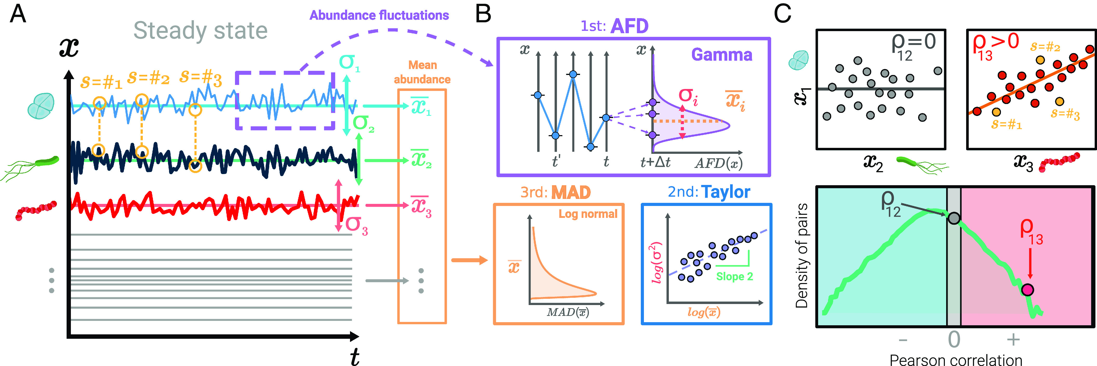
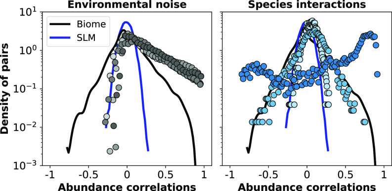
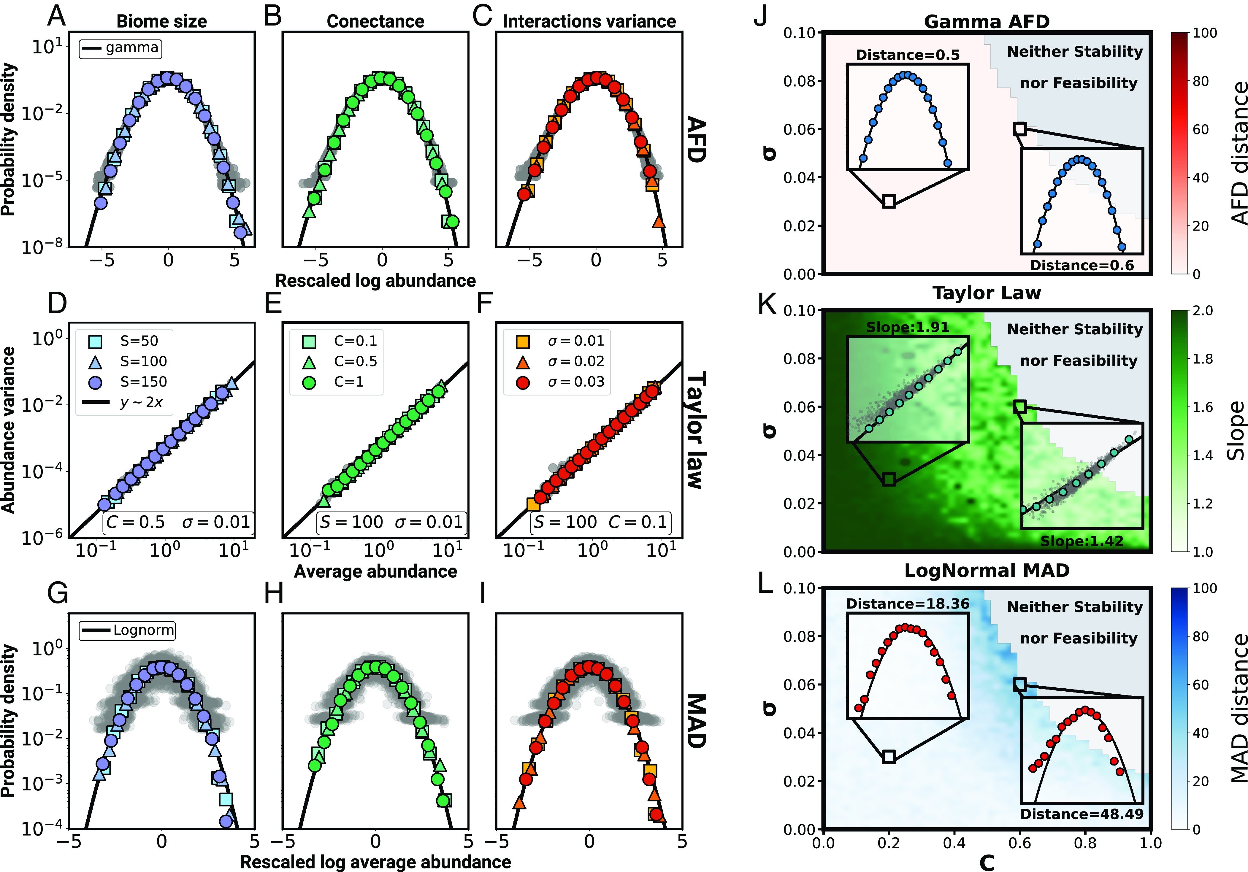
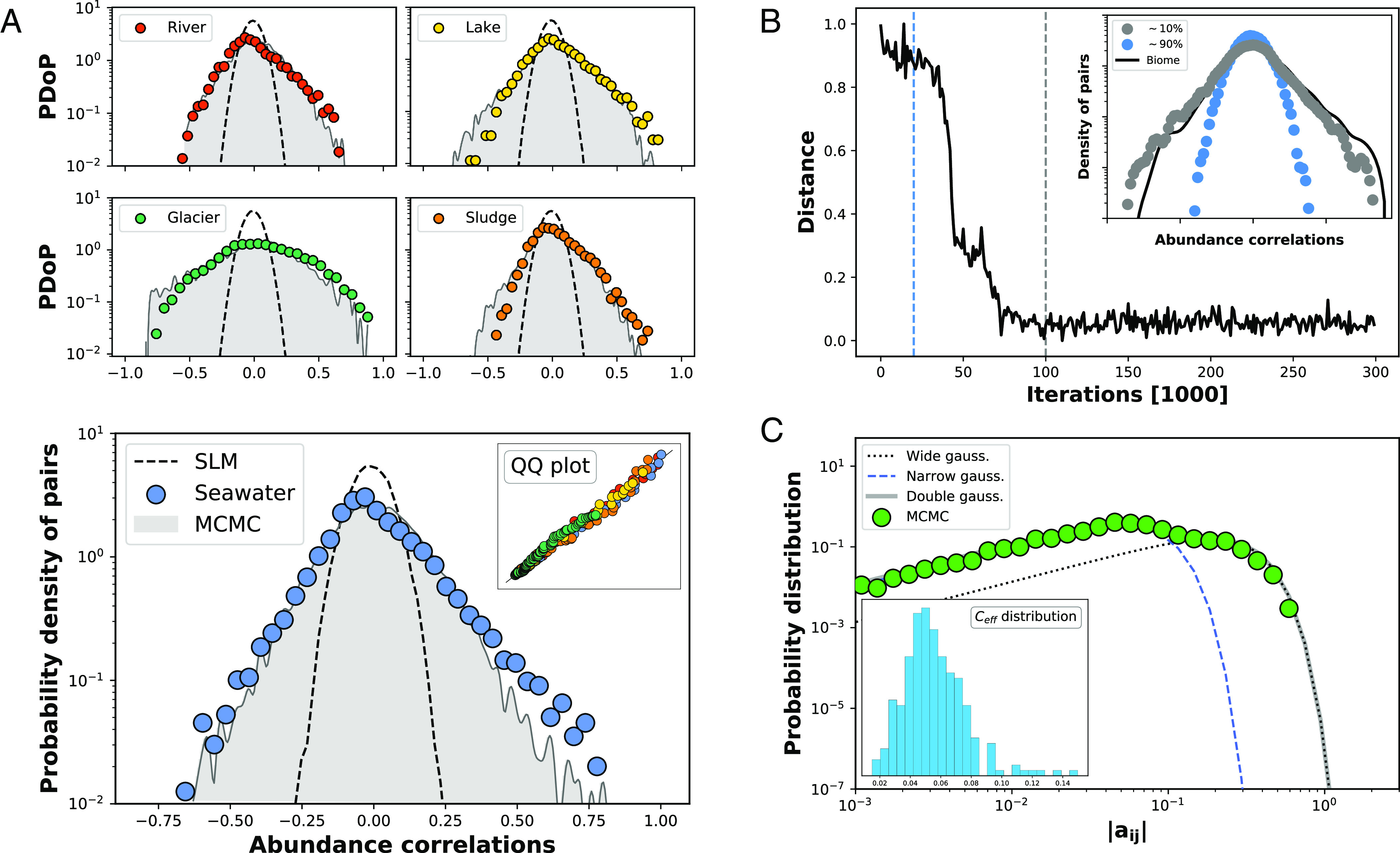
During the last decades, macroecology has identified broad-scale patterns of abundances and diversity of microbial communities and put forward some potential explanations for them. However, these advances are not paralleled by a full understanding of the dynamical processes behind them. In particular, abundance fluctuations of different species are found to be correlated, both across time and across communities in metagenomic samples. Reproducing such correlations through appropriate population models remains an open challenge. The present paper tackles this problem and points to sparse species interactions as a necessary mechanism to account for them. Specifically, we discuss several possibilities to include interactions in population models and recognize Lotka-Volterra constants as a successful ansatz. For this, we design a Bayesian inference algorithm to extract sets of interaction constants able to reproduce empirical probability distributions of pairwise correlations for diverse biomes. Importantly, the inferred models still reproduce well-known single-species macroecological patterns concerning abundance fluctuations across both species and communities. Endorsed by the agreement with the empirically observed phenomenology, our analyses provide insights into the properties of the networks of microbial interactions, revealing that sparsity is a crucial feature.

Keywords: Lotka–Volterra; correlations; ecology; interactions; microbiome.

Fig. 1.

Infographic of the population dynamics and the resulting macroecological patterns. Panel (A) portrays, as an illustrative example, three individual-species (color coded) time courses at equally spaced times (longitudinal data), resulting from the integration of Eq. 1. The abundances at different samples describe the fluctuations around the mean (abundance fluctuation distribution, AFD) are well described by a gamma distribution, as shown in panel (B) (SI Appendix, Figs. S4 and S5). For each species, this distribution is characterized by its mean value ${\overline{x}}_i$ and its variance ${\sigma }_i^2$. These two magnitudes are linked by Taylor’s law ${\sigma }_i^2\propto {\overline{x}}_i^2$ [panel (B)]. The mean abundances of all species are distributed as a lognormal (mean abundance distribution, MAD), panel (B). Further details about Taylor’s law and MAD are presented in SI Appendix, Figs. S6 and S7. Panel (C) illustrates the correlations between abundance fluctuations of pairs of species across samples (a point for each sample/realization). The Top-Left plot illustrates the case of two uncorrelated species, whereas the Top-Right plot illustrates two positively correlated species. The Bottom picture shows the distribution of Pearson’s coefficients ${\rho }_{\mathit{ij}}$ of all pairs of species. Empirically, this distribution is found to generally cover the entire range $-1\le {\rho }_{\mathit{ij}}\le 1$ and to exhibit a peak at negative values.

Fig. 2.

Distributions of Pearson’s abundance correlation coefficients as obtained in the model with (Left panel) a few samples of the noise correlation matrix $\mathbf{W}$ (each with a different gray shade) or (Right panel) with random samples of the Lotka–Volterra matrix $\mathbf{A}$. The black solid lines portray in each case, the empirical distribution as obtained from the Seawater microbiome (species which appear in less than 50% of the communities have been filtered out), while the blue ones represent the distribution of correlations as obtained from the model without interactions. In the Left plot, colored circles show the results for a few samples of matrices $\mathbf{W}$ (see “Material and Methods” for details of the sampling procedure); Lotka–Volterra constants are chosen as $a_{\mathit{ij}}=-{\delta }_{\mathit{ij}}/K_i$, with carrying capacities $K_i$ sampled from a lognormal distribution with mean $0.1$ and SD $0.5$—as for the SLM (15). The results shown in this figure are typical (SI Appendix, sections 7B and C for a more thorough exploration). In the Right plot, colored circles represent correlations resulting from the SLVM with $\mathbf{W}=w\mathbf{I}$ and Lotka–Volterra constants $a_{\mathit{ij}}$ ($i\ne j$) sampled from a Gaussian distribution with zero mean and SD $0.03$. A random selection of $60\%$ of such constants are set to zero (i.e., the connectance of the interaction matrix is $C=0.4$).

Fig. 3.

Grilli’s three macroecological laws as a function of the interaction parameters. Specifically, the figure shows the abundance fluctuation distribution (AFD) (panels A–C), Taylor’s law (panels D–F), and the MAD, (panels G–I) for different values of the species number $S$ (panels A, D, and G), the connectance $C$ (panels B, E, and H), and SD of the interaction constants $\sigma$ (panels C, F, and I). Results have been averaged over $100$ realizations of the SLVM Eq. 1 each one with a different random interaction matrix. Results including all realizations are depicted as a cloud of gray points, whereas averages are shown as colored bullets. The AFD obtained for a given realization contains the results for all species, represented in terms of rescaled logarithm abundances ($z=\mathrm{Var}{(x)}^{-1/2}log(x/\overline{x})$). Solid black lines correspond to gamma distributions. MAD plots (G–I) is obtained by properly rescaling the mean abundances and are fitted by a normalized (zero mean, unit SD) lognormal distribution (black solid line). Similarly, the black straight lines in (panels D–F) describe the relation $\mathrm{Var}(x_i)\propto {\overline{x}}_i^2$ in logarithmic scale. (Panels J–L) illustrate the limits of the weak-interaction regime across the set of parameters that characterize species interactions. The plots quantify the compliance with (J) a gamma AFD, (K) Taylor’s law, and (L) a lognormal MAD, within the region where the system is stable and feasible. Each pixel corresponds to a combination of values of the network connectance $C$ (horizontal axis) and the SD $\sigma$ of the distribution of interactions (vertical axis). The color of the pixel quantifies the distance from the AFD to a gamma distribution (J), the value of the exponent $\gamma$ in the relationship $\mathrm{Var}(x_i)\propto {\overline{x}}_i^{\gamma }$ (K), and the distance of the MAD to a lognormal distribution (L), averaged over a sample of $100$ realizations. Gray areas mark the region of the parameter space where the resulting systems are neither stable nor feasible. In these plots $S=50$, ${\tau }_i=0.1$, $w=0.1$, and the carrying capacities are sampled from a lognormal distribution (mean $0.1$, SD $0.5$).

Fig. 4.

Abundance correlation distributions for real and simulated communities. In (A), different colored bullets correspond to different biomes selected from the EBI metagenomics platform (45) (namely Seawater, River, Lake, Glacier, and Sludge communities). Black dashed lines portray the distribution of Pearson’s coefficients for the abundance correlation of all pairs of species resulting from the SLM. Gray curves show the same distributions as obtained from the SLVM, c.f., Eq. 1, with the Lotka–Volterra interaction constants inferred using the Bayesian approach described in “Material and Methods.” The Inset in the Bottom panel of (A) presents the quantile–quantile (QQ) plot, comparing quantiles of the empirical and the synthetic distributions, for the different biomes. The dots sit on the bisector line, indicating the close alignment between the quantiles of both distributions for each single biome. This test is consistent with the results of a Kolmogorov–Smirnov test ($P$-values of Seawater and River: $0.99$; Lake and Glacier: $0.90$; Sludge: $0.81$). The Top panel of (B) shows the Euclidean distance between the logarithms of the empirical and the synthetic distributions (for Seawater, using only species appearing in at least 50% of the samples) vs. the iterations of the MCMC. In blue and gray dots, the Inset shows the synthetic distributions obtained at the iteration marked by a dashed line of the corresponding color. The empirical distribution is drawn with a solid black line. (C) shows the distribution of absolute values of the interaction constants ($|a_{\mathit{ij}}|$) for a collection of over $200$ matrices generated through the MCMC method (green bullets). This distribution can be fitted by a convex combination of two Gaussian distributions (gray solid line). The black (blue) dashed line fits the broader (narrower) Gaussian. Practically all coefficients in the narrower Gaussian are negligible compared to the broader one. Hence, the presence of a small fraction of large coefficients gives rise to an effective connectance ($C_{\text{eff}}$) in the associated network. The Inset shows a histogram of the values of $C_{\text{eff}}$. It peaks around $0.05$, with tails extending approximately in the range $0.01\lesssim C_{\text{eff}}\lesssim 0.15$. This reveals the high sparsity of the interactions.

References

-
- Handelsman J., Rondon M. R., Brady S. F., Clardy J., Goodman R. M., Molecular biological access to the chemistry of unknown soil microbes: A new frontier for natural products. Chem. Biol. 5, R245–R249 (1998). - PubMed
- Steele H. L., Streit W. R., Metagenomics: Advances in ecology and biotechnology. FEMS Microbiol. Lett. 247, 105–111 (2005). - PubMed
- Rappé M. S., Giovannoni S. J., The uncultured microbial majority. Annu. Rev. Microbiol. 57, 369–394 (2003). - PubMed
- Hug L. A., et al. , A new view of the tree of life. Nat. Microbiol. 1, 16048 (2016). - PubMed
MeSH terms
Grants and funding
- PGC2018-098186-B-I00/Ministerio de Ciencia e Innovación (MCIN)
- PID2021-128966NB-I00/Ministerio de Ciencia e Innovación (MCIN)
- PID2020-113681GB-I00/Ministerio de Ciencia e Innovación (MCIN)
- B-FQM-366-UGR20/Consejería de Conocimiento, Investigación y Universidad, Junta de Andalucía (Ministry of Knowledge, Research and University, Andalusia)
- PGC2022-141802NB-I00/Ministerio de Ciencia e Innovación (MCIN)
LinkOut - more resources
Full Text Sources