Increasing the accuracy of single-molecule data analysis using tMAVEN

Abstract

Time-dependent single-molecule experiments contain rich kinetic information about the functional dynamics of biomolecules. A key step in extracting this information is the application of kinetic models, such as hidden Markov models (HMMs), which characterize the molecular mechanism governing the experimental system. Unfortunately, researchers rarely know the physicochemical details of this molecular mechanism a priori, which raises questions about how to select the most appropriate kinetic model for a given single-molecule data set and what consequences arise if the wrong model is chosen. To address these questions, we have developed and used time-series modeling, analysis, and visualization environment (tMAVEN), a comprehensive, open-source, and extensible software platform. tMAVEN can perform each step of the single-molecule analysis pipeline, from preprocessing to kinetic modeling to plotting, and has been designed to enable the analysis of a single-molecule data set with multiple types of kinetic models. Using tMAVEN, we have systematically investigated mismatches between kinetic models and molecular mechanisms by analyzing simulated examples of prototypical single-molecule data sets exhibiting common experimental complications, such as molecular heterogeneity, with a series of different types of HMMs. Our results show that no single kinetic modeling strategy is mathematically appropriate for all experimental contexts. Indeed, HMMs only correctly capture the underlying molecular mechanism in the simplest of cases. As such, researchers must modify HMMs using physicochemical principles to avoid the risk of missing the significant biological and biophysical insights into molecular heterogeneity that their experiments provide. By enabling the facile, side-by-side application of multiple types of kinetic models to individual single-molecule data sets, tMAVEN allows researchers to carefully tailor their modeling approach to match the complexity of the underlying biomolecular dynamics and increase the accuracy of their single-molecule data analyses.

Figure 1

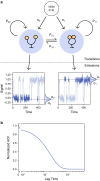
Molecular mechanisms and their corresponding single-molecule signal versus time trajectories. (Top) Schematic of the molecular mechanism, (middle) the corresponding conformational free-energy landscape, and (bottom) single-molecule trajectories that capture changes in signal for reaction coordinate 1 for (a) homogeneous, (b) statically heterogeneous, and (c) dynamically heterogeneous biomolecular systems. Simulated random walkers on the conformational free-energy landscape, starting at circles and ending at arrows, show hypothetical individual molecules undergoing transitions that correspond to the gray areas of the single-molecule trajectories. For the heterogeneous cases, blue and red correspond, respectively, to slow- and fast-transitioning subpopulations (for static) and phases (for dynamic), which are differentiated along reaction coordinate 2. A discontinuity (hatched line) is shown in the landscape for (b) to signify the lack of allowed transition along reaction coordinate 2 in this case. To see this figure in color, go online.

Figure 2

Schematic diagram of a kinetic model. (a) A schematic diagram of a two-state HMM showing the separation between the transition DoFs comprised of the initial probabilities and the transition probabilities, and the emission DoFs comprised of the emission probability distributions. (b) The normalized ACF corresponding to the HMM in (a) expresses all the dynamics of the kinetic model from both the transitions and the emissions in a single analytical form. To see this figure in color, go online.

Figure 3

Comparisons of ACFs for homogeneous ensembles. (a) (Top) The true ACF for the homogenous data set (solid black) along with the mean of the ACFs (dashed blue) calculated using HMMs inferred from 100 ensembles using composite HMMs (left) and global HMMs (right), along with (bottom) the corresponding mean (dashed blue) of the residuals of the inferred ACFs to the true ACF. The blue area denotes the region one standard deviation away from the mean across 100 homogeneous ensembles. The gray dashed line corresponds to zero. (b) The true (black) and model (blue) ACFs, along with the means of the residuals (blue), inferred using composite (left) and global (right) HMMs for homogeneous data sets of signal versus time trajectories of varying lengths (top) and varying numbers (bottom). The blue area denotes the region one standard deviation away from the mean across 100 homogeneous ensembles. The gray dashed line corresponds to zero. To see this figure in color, go online.

Figure 4

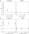
The effects of the lengths and number of trajectories in a mesoscopic ensemble on kinetic modeling. The transition probabilities from the “0” state to the “1” observed states inferred using (left) composite HMMs and (right) global HMMs from homogenous data sets with (a) varying lengths of trajectories and (b) varying numbers of trajectories. The dashed line represents the true transition probability for the data set. The transition probabilities from the “1” state to the “0” state follow the same trend (data not shown). Error bars represent standard deviations of the estimated transition probabilities across 100 homogeneous ensembles. To see this figure in color, go online.

Figure 5

The effects of static heterogeneity on kinetic modeling. (Left) Kernel density estimated distributions of the transition probabilities for the observed “open” and “closed” states inferred from the individual trajectory-level HMMs for each molecule in mesoscopic ensembles with varying amounts of static heterogeneity. Dashed red and blue lines denote the transition probabilities from each state for the subpopulation of fast- and slow-transitioning molecules, respectively. (Middle) The ensemble-level transition probabilities for the observed states inferred using global HMMs as a function of the average transition probability of the observed states (calculated using the proportions of fast- and slow-transitioning molecules). The dashed gray line denotes identity. (Right) The two transition probabilities for each observed state as inferred using a hierarchical HMM as a function of the average transition probability of the observed states calculated using the proportions of fast and slow subpopulations. Error bars represent standard deviations of the estimated transition probabilities across 100 statically heterogeneous ensembles. To see this figure in color, go online.

Figure 6

The effects of dynamic heterogeneity on kinetic modeling. (Left) Kernel density estimated distributions of the transition probabilities for the observed “open” and “closed” states inferred by the individual trajectory-level HMMs for each molecule in mesoscopic ensembles with varying total probability of transition between slow- and fast-transitioning phases (P_sf + P_fs). Dashed red and blue lines denote the transition probabilities of each state for the fast- and slow-transitioning phases, respectively. The dashed gray line denotes the ensemble average transition probability of each observed state. (Middle) The ensemble-level transition probabilities for the observed states inferred using global HMMs as a function of the total probability of transition between slow- and fast-transitioning phases. (Right) The two transition probabilities for each observed state inferred using hierarchical HMMs as a function of the total probability of transition between slow- and fast-transitioning phases. Error bars represent standard deviations of the estimated transition probabilities across 100 dynamically heterogeneous ensembles. To see this figure in color, go online.

References

1. Bustamante C., Bryant Z., Smith S.B. Ten years of tension: single-molecule DNA mechanics. Nature. 2003;421:423–427. - PubMed
1. Tinoco I., Gonzalez R.L. Biological mechanisms, one molecule at a time. Genes Dev. 2011;25:1205–1231. - PMC - PubMed
1. MacDougall D.D., Fei J., Gonzalez R.L. In: Molecular Machines in Biology. Frank J., editor. Cambridge University Press; Cambridge: 2011. Single-Molecule Fluorescence Resonance Energy Transfer Investigations of Ribosome-Catalyzed Protein Synthesis; pp. 93–116.
1. Kinz-Thompson C.D., Ray K.K., Gonzalez R.L. Bayesian Inference: The Comprehensive Approach to Analyzing Single-Molecule Experiments. Annu. Rev. Biophys. 2021;50:191–208. - PMC - PubMed
1. Du C., Kou S.C. Statistical Methodology in Single-Molecule Experiments. Stat. Sci. 2020;35:75–91.
LinkOut - more resources