Multi-region calcium imaging in freely behaving mice with ultra-compact head-mounted fluorescence microscopes

Abstract

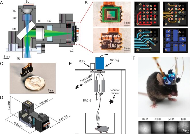
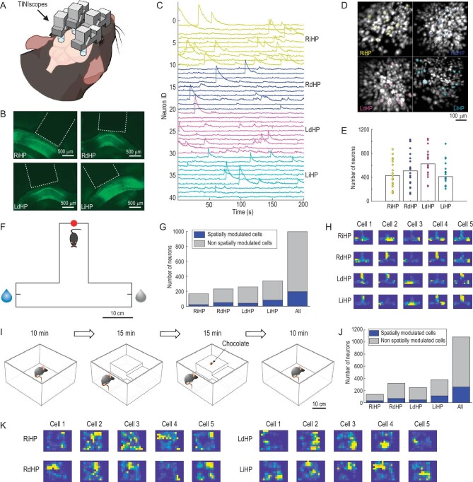
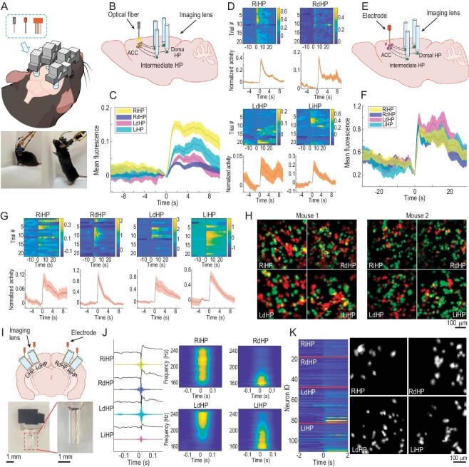
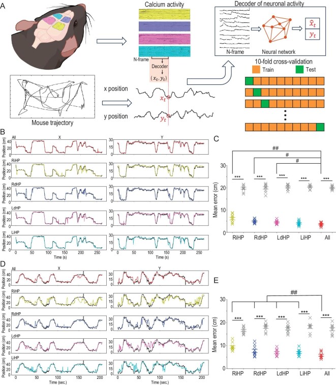
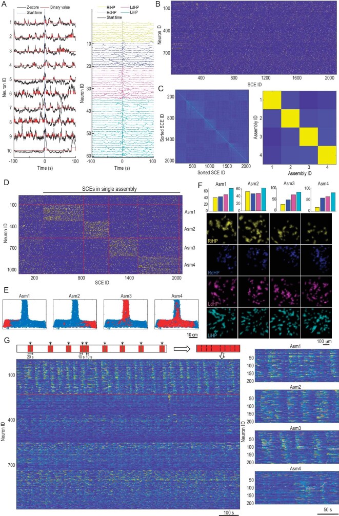
To investigate the circuit-level neural mechanisms of behavior, simultaneous imaging of neuronal activity in multiple cortical and subcortical regions is highly desired. Miniature head-mounted microscopes offer the capability of calcium imaging in freely behaving animals. However, implanting multiple microscopes on a mouse brain remains challenging due to space constraints and the cumbersome weight of the equipment. Here, we present TINIscope, a Tightly Integrated Neuronal Imaging microscope optimized for electronic and opto-mechanical design. With its compact and lightweight design of 0.43 g, TINIscope enables unprecedented simultaneous imaging of behavior-relevant activity in up to four brain regions in mice. Proof-of-concept experiments with TINIscope recorded over 1000 neurons in four hippocampal subregions and revealed concurrent activity patterns spanning across these regions. Moreover, we explored potential multi-modal experimental designs by integrating additional modules for optogenetics, electrical stimulation or local field potential recordings. Overall, TINIscope represents a timely and indispensable tool for studying the brain-wide interregional coordination that underlies unrestrained behaviors.

Keywords: calcium imaging; hippocampus; miniature microscope; multimodal integration; multiple sites.

Figure 1.

Tightly integrated neuronal imaging fluorescence microscope (TINIscope). (A) Section diagram of TINIscope. BL, blue LED; HL, half-ball lens; ExF, excitation filter; DM, dichroic mirror; GL, GRIN objective lens; CL, convex lens; EmF, emission filter; CC, CMOS camera. (B) Photos of an image sensor with HDI rigid PCB and layout of stacked layers (from top to bottom layer: red, brown, cyan and blue) with blind and buried vias (bicolor). (C) Photo of TINIscope and a nickel shown for scale. (D) Dimensions of TINIscope. (E) Schematic diagram of the experimental system with TINIscope. (F) Top: photo of a mouse with four head-mounted TINIscopes. Bottom: simultaneously recorded images of 4 hippocampal subregions.

Figure 2.

Simultaneous calcium imaging of 4 hippocampal subregions in different behavioral experiments. (A) Diagram of 4-region recordings in mice. (B) Fluorescence images of brain slices around the four recorded hippocampal subregions. The white dashed lines indicate GRIN lenses. (C) Calcium traces of example neurons from the RiHP (yellow), RdHP (blue), LdHP (magenta), and LiHP (cyan). (D) The spatial contours of example neurons in (C) and the corresponding maximum intensity map (MIP) of the background-subtracted videos. (E) Number of identified neurons in all sessions and their averages (n = 20 sessions, 6 mice). (F) Paradigm of the T-maze task. The water reward was given at a random end in each trial. Red dot: start point; blue droplet: reward side; gray droplet: non-reward side. (G) The proportion of spatially modulated cells during the T-maze task. (H) Place fields of example spatially modulated cells in the T-maze box. (I–K) same as (F–H) but the mouse was in an open field exploration experiment. The mouse explored freely in an open field with changing environments.

Figure 3.

Combination of optogenetic/electrophysiological modules and TINIscope. (A) Top: diagram of potential experimental paradigms that combine multiple-TINIscope imaging and other technique modules, as listed in the dashed box (optogenetics, electrical stimulation and electrophysiological recordings). Bottom: photos of mice carrying 4 TINIscopes together with two electrical stimulating electrodes (left) or four extracellular recording electrodes (right). (B) Diagram investigating the ACC-HP circuit by combining optogenetics with 4-region TINIscope imaging. (C) Mean of the background-subtracted fluorescence signals averaged over all left-ACC stimulation trials (n = 21 trials, 1 mouse, t = 0 indicates the stimulation onset). (D) Normalized activity of example ACC-responsive neurons in different trials (top) and the corresponding mean activity over trials (bottom). The traces were normalized using the estimated noise level and centered around the value at the onset of stimulation (t = 0). (E–G) same as (B–D) but replacing optogenetic stimulation with electrical stimulation (n = 42 trials, 2 mice). (H) Left: spatial footprints of neurons responding to left (red) or right (green) ACC stimulation, respectively; right: same as the left but with the other mouse. (I) Top: illustration of joint calcium imaging and LFP recording in four hippocampal subregions. Bottom: photo of the electrode-lens complex. (J) Raw LFP and filtered signals (150–250 Hz) when all four regions show SWRs together. Right, spectrograms of LFP signals in four regions. (K) Synchronous calcium traces (left) and their spatial footprints (right) concurrent with the SWR in (J). Shaded areas in (C, D, F, J) correspond to the mean ± s.e.m.

Figure 4.

Decoding mouse position from extracted neuronal traces. (A) Schematic illustration of machine-learning–based decoders for predicting mouse position from neuronal activity. Bottom right: the extracted calcium traces were split into 10 folds, and one testing fold was sequentially chosen to calculate the decoding error with the decoder trained from the remaining 9 folds. Decoding the position at each time point requires the population neuronal activity of the previous N (here, N = 5) frames. The LSTM network was used as the decoding model in this work. (B) Example of decoded mouse positions (color lines) on testing data and the true position (black lines) in the T-maze experiment. The number of temporal bins in this testing fold is 2670 (bin size = 100 ms). (C) The mean decoding error using different sets of neuronal traces in the T-maze experiment. Gray data points correspond to the chance level decoding errors where the mouse positions were randomly shuffled. ***P < 0.001, Mann–Whitney test, n = 10 folds, 1 mouse. ^##P < 0.01, ^#P < 0.05, Wilcoxon matched-pairs sign rank test, n = 10 folds, 1 mouse. The results show the mean ± s.e.m. (D and E) same as (B and C) but the mouse was in the open field experiment (temporal bins = 2059).

Figure 5.

Neuronal assemblies during the T-maze task. (A) Detection of SCEs from extracted calcium traces. Left: activities of the example neurons were z-scored and thresholded at 1 standard deviation (SD); right, neuronal activity of all neurons participating in an SCE. The vertical lines indicate the onset of an SCE. (B) Raster plot of neuronal participation in all SCEs. (C) Correlation maps of the detected SCEs (left) and the identified neuronal assemblies (right). The SCE IDs were ordered by the associated assemblies of the participating neurons in each SCE. (D) Same as (B) but the neuron IDs and SCE IDs were ordered to match the found assemblies. The SCEs to the left column were not involved in any assembly, while the SCEs to the right column were involved in multiple assemblies. (E) The mouse's position when SCEs associated with a specific assembly occurred. (F) The number of neurons in each region (color coded as labels below) and their spatial footprints in different assemblies. (G) Neurons associated with each assembly showed repeated activation sequences. Left is the concatenated calcium traces, as illustrated in the top diagram. Only time intervals within ± 10 second windows of all SCEs associated with an example assembly (assembly 3, including neurons above the red line) will be preserved. Neurons were grouped by their associations with different assemblies. Within each assembly, neuron IDs were sorted according to their peak intensity time. Right, repeated activation sequences of neurons associated with each assembly.

References

1. Abbott LF, Angelaki DE, Carandini M et al. An international laboratory for systems and computational neuroscience. Neuron 2017; 96: 1213–8.10.1016/j.neuron.2017.12.013 - DOI - PMC - PubMed
1. Machado TA, Kauvar IV, Deisseroth K. Multiregion neuronal activity: the forest and the trees. Nat Rev Neurosci 2022; 23: 683–704.10.1038/s41583-022-00634-0 - DOI - PMC - PubMed
1. Wang X-J. Theory of the multiregional neocortex: large-scale neural dynamics and distributed cognition. Annu Rev Neurosci 2022; 45: 533–60.10.1146/annurev-neuro-110920-035434 - DOI - PMC - PubMed
1. Allen WE, Chen MZ, Pichamoorthy N et al. Thirst regulates motivated behavior through modulation of brainwide neural population dynamics. Science 2019; 364: eaav3932.10.1126/science.aav3932 - DOI - PMC - PubMed
1. Harvey RE, Robinson HL, Liu C et al. Hippocampo-cortical circuits for selective memory encoding, routing, and replay. Neuron 2023; 111: 2076–90.10.1016/j.neuron.2023.04.015 - DOI - PMC - PubMed