Improved atmospheric constraints on Southern Ocean CO2 exchange

Abstract

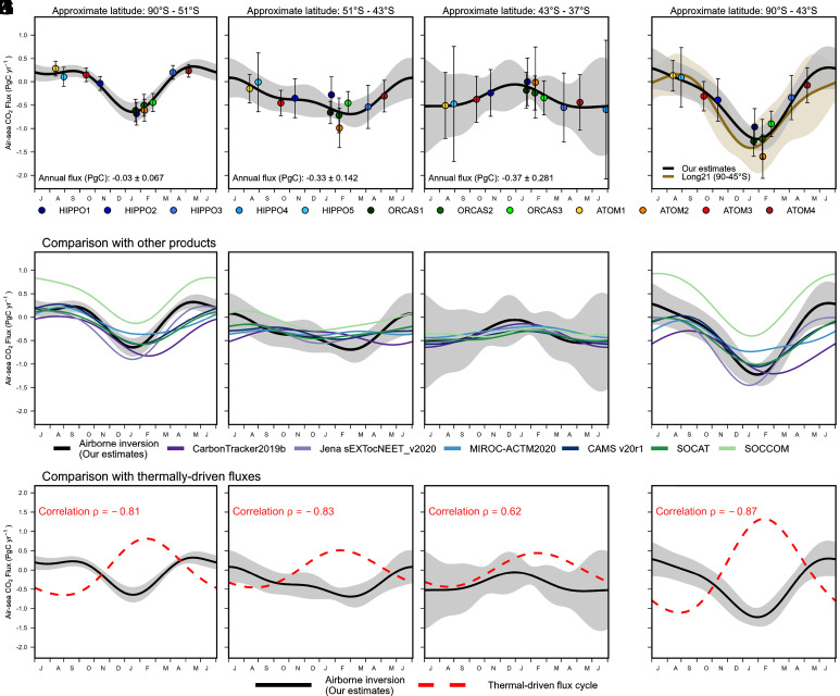
We present improved estimates of air-sea CO₂ exchange over three latitude bands of the Southern Ocean using atmospheric CO₂ measurements from global airborne campaigns and an atmospheric 4-box inverse model based on a mass-indexed isentropic coordinate (M_θe). These flux estimates show two features not clearly resolved in previous estimates based on inverting surface CO₂ measurements: a weak winter-time outgassing in the polar region and a sharp phase transition of the seasonal flux cycles between polar/subpolar and subtropical regions. The estimates suggest much stronger summer-time uptake in the polar/subpolar regions than estimates derived through neural-network interpolation of pCO₂ data obtained with profiling floats but somewhat weaker uptake than a recent study by Long et al. [Science 374, 1275-1280 (2021)], who used the same airborne data and multiple atmospheric transport models (ATMs) to constrain surface fluxes. Our study also uses moist static energy (MSE) budgets from reanalyses to show that most ATMs tend to have excessive diabatic mixing (transport across moist isentrope, θ_e, or M_θe surfaces) at high southern latitudes in the austral summer, which leads to biases in estimates of air-sea CO₂ exchange. Furthermore, we show that the MSE-based constraint is consistent with an independent constraint on atmospheric mixing based on combining airborne and surface CO₂ observations.

Keywords: airborne observation; atmospheric diabatic mixing; atmospheric transport model; carbon sink; inverse model.

Fig. 1.

(A) Schematic of the box model. Boundaries of the box model are selected M_θe surfaces at 15, 30, 45, and 60 M_θe values (10¹⁶ kg), which are shown as zonal and 2009 to 2018 averages. (B) Selected near-surface M_θe contours as 2009 to 2018 averages. M_θe is computed from 3-h MERRA-2 reanalysis. These M_θe bands are nearly fixed with season (SI Appendix, Fig. S2). Red triangles show the location of surface stations that are used in the Carbon Tracker 2019b 3D (three-dimensional) CO₂ inversion product.

Fig. 2.

(A) Monthly reconstructed air–sea CO₂ fluxes (solid gray) for the 0 to 30 (10¹⁶ kg) M_θe band (south of ~43°S near the Earth surface) based on CarbonTracker 2019b, compared with the original monthly 3D inversion fluxes for the same M_θe band (dashed black). The other components (i.e., diabatic CO₂ transport and CO₂ inventory change, detailed in Materials and Methods, and Eq. 1) of the box-model reconstruction are shown as well. Positive values of the diabatic transport represent CO₂ transport into the 0 to 30 M_θe band (poleward transport). We note that the inventory change (blue) equals the sum of fluxes (black) and diabatic transport (red). (B) Similar to (A), but showing the flux and other components as climatological monthly averages (2009 to 2018). Shaded regions show IAV, which is calculated as the SD over 10 y for the corresponding month. We also show these reconstructions for other 3D inversion products and other surface M_θe bands in SI Appendix, Figs. S4–S6.

Fig. 3.

Diabatic mixing rates of the 30 (10¹⁶ kg) M_θe surface. These mixing rates are parameterized from four 3D CO₂ inversion products and MSE budget of two reanalysis products (MERRA-2 and JRA-55). Error bars represent only the IAV of parameterized mixing rates, which is shown to be small, with the exception of CAMS in September because of the close-to-zero CO₂ gradient across the 30 (10¹⁶ kg) M_θe surface. Diabatic mixing rates of the 15 and 45 (10¹⁶ kg) M_θe surface are shown in SI Appendix, Fig. S3.

Fig. 4.

Exploring the correlation between January and February ATM-based mixing rates at (A) the 15 M_θe surface, (B) the 30 M_θe surface, and (C) the 45 M_θe surface and simulated atmospheric CO₂ gradients across the corresponding M_θe surface of four transport models (3D CO₂ inversion products). Simulated gradients are from 3D concentration fields averaged at the mean dates of five airborne campaigns or subcampaigns that took place during January and February (HIPPO1, ATom2, and ORCAS1-3). The corresponding ATM-based mixing rate is calculated as the January and February average. For comparison, we show the observed CO₂ gradients (spatial bias corrected, as detailed in SI Appendix, Text S1) as horizontal black lines, which are calculated as the average of the same five campaigns or subcampaigns, while the dashed lines show the 1 $\sigma$ uncertainty (measurement and spatial bias correction uncertainty). We also show two MSE-based mixing rates (January and February average) as vertical brown lines. A similar figure exploring the correlation between April to November averaged CO₂ gradient and averaged diabatic mixing rate is presented in SI Appendix, Fig. S7.

Fig. 5.

(A–D) Seasonal cycle of air–sea CO₂ fluxes (negative as net oceanic uptake) estimated using the 4-box model based on airborne CO₂ observations and two sets of MSE-based diabatic mixing rates (Materials and Methods). Each individual point represents the calculated fluxes using airborne observations from the corresponding campaign, centering on the mean date of each campaign, while the black line is a 2-harmonic fit. Error bars represent the 1 $\sigma$   uncertainty of each flux estimate, while shaded regions represent the 1 $\sigma$   uncertainty of the 2-harmonic fits (detailed in SI Appendix, Texts S1 and S2). Values of air–sea CO₂ fluxes calculated for each airborne campaign transect and for each band are summarized in SI Appendix, Table S4. Annual fluxes are from the constant term of the 2-harmonic fitted climatological flux cycles, which is equivalent to integrating the fit over a year. These approximate latitude bands (see the Top of each panel) are calculated as the zonal average latitude of the corresponding annual average (2009 to 2018) M_θe surface over the ocean (SI Appendix, Fig. S2). We also show box-model resolved fluxes calculated using the average of six sets of mixing rates and each set of mixing rate in SI Appendix, Figs. S10 and S11. In (E–H), we compare our estimates with four 3D CO₂ inversion products, and two neural network interpolated surface ocean pCO₂ products using SOCAT pCO₂ observations alone and SOCCOM pCO₂ observations alone. Details of these products are in SI Appendix, Text S6. The SOCCOM product is a sensitivity run where all shipboard data from SOCAT were excluded (only SOCCOM float data were included). We note that the ocean CO₂ flux in Jena sEXTocNEET_v2020 is a prior, which is provided by assimilation of surface ocean pCO₂ observations (i.e., not neural-network derived pCO₂) from SOCAT (29) by the Jena mixed-layer scheme (46). The seasonal cycle of each product is calculated as the average between 2009 and 2018, except for SOCCOM, which is averaged from 2015 to 2017. In (I–L), we compare our estimates with thermally driven air–sea CO₂ flux cycles (dashed red, methods in SI Appendix, Text S3), which is derived from assuming 4% pCO₂ increase per degree Celsius increase in sea-surface temperature (SST) and using wind speed–dependent gas exchange. We calculate the correlation between the airborne observed flux cycle and the estimated thermal-driven flux cycle of each band. Black solid curves and shaded regions in (E–L) are corresponding airborne observed fluxes and 1σ uncertainty. Panels (I–L) have a different y-axis range compared to panels (A–H). We also compare our estimates with nine global ocean biogeochemistry models that are used in the Global Carbon Budget 2020 (10, 47) in SI Appendix, Fig. S9.

References

1. Gruber N., et al. , The oceanic sink for anthropogenic CO2 from 1994 to 2007. Science 363, 1193–1199 (2019). - PubMed
1. Hauck J., et al. , On the Southern Ocean CO2 uptake and the role of the biological carbon pump in the 21st century. Global Biogeochem. Cycles 29, 1451–1470 (2015).
1. Kessler A., Tjiputra J., The Southern Ocean as a constraint to reduce uncertainty in future ocean carbon sinks. Earth Syst. Dyn. 7, 295–312 (2016).
1. Lovenduski N. S., McKinley G. A., Fay A. R., Lindsay K., Long M. C., Partitioning uncertainty in ocean carbon uptake projections: Internal variability, emission scenario, and model structure. Global Biogeochem. Cycles 30, 1276–1287 (2016).
1. Gloor M., et al. , A first estimate of present and preindustrial air-sea CO2 flux patterns based on ocean interior carbon measurements and models. Geophys. Res. Lett. 30, 10-1–10-4 (2003).