The Hopf whole-brain model and its linear approximation

Abstract

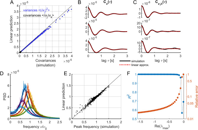
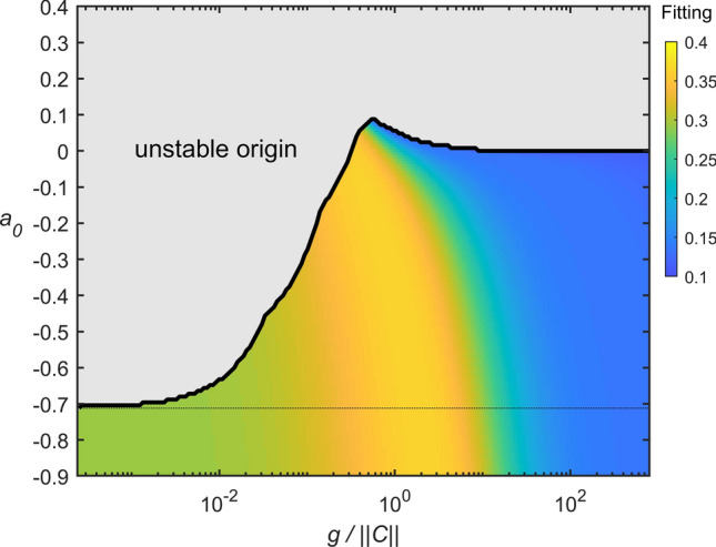
Whole-brain models have proven to be useful to understand the emergence of collective activity among neural populations or brain regions. These models combine connectivity matrices, or connectomes, with local node dynamics, noise, and, eventually, transmission delays. Multiple choices for the local dynamics have been proposed. Among them, nonlinear oscillators corresponding to a supercritical Hopf bifurcation have been used to link brain connectivity and collective phase and amplitude dynamics in different brain states. Here, we studied the linear fluctuations of this model to estimate its stationary statistics, i.e., the instantaneous and lagged covariances and the power spectral densities. This linear approximation-that holds in the case of heterogeneous parameters and time-delays-allows analytical estimation of the statistics and it can be used for fast parameter explorations to study changes in brain state, changes in brain activity due to alterations in structural connectivity, and modulations of parameter due to non-equilibrium dynamics.

Figure 1

Hopf model: single-node and network dynamics. (A) The fixed points of a Hopf node have modules which are the roots of $\dot{r}=ar-r^3$. For $a<0$, the solution $r=0$ is stable since deviations from $r=0$ are attenuated (i.e., $\dot{r}<0$). On the contrary, if $a>0$, $r=0$ is unstable as fluctuations around it are amplified (i.e., $\dot{r}>0$). In this latter case a new fixed point appears given by $r=a^{1/2}$, which is stable since fluctuations around it, $r=a^{1/2}+\delta r$, are increased if $\delta r<0$, but decreased if $\delta r>0$. The arrows indicate the direction of flow and are given by the sign of $\dot{r}$. (B) Single-node dynamics for $a<0$. The system relaxes with damped oscillations from the initial condition (white circle) to the origin of the complex plane. Insets: top: in the absence of noise ($\eta =0$) the oscillations die out; bottom: in the presence of noise ($\eta \ne 0$) the oscillations are noise-driven. (C) Single-node dynamics for $a>0$. The system produces self-sustained oscillations. Insets: top, deterministic system; bottom, stochastic system. (D) Network model. The whole-brain network is composed of $N$ Hopf nodes interconnected through anatomical connections. Here, we used dMRI connectivity from the Human Connectome Project (HCP), in a parcellation with $N$ = 1000 nodes. (E) Example dynamics for five nodes of the network. Parameters: $a_j=-0.5$ (homogeneous); $g=1$; ${\omega }_j=10$ rad.s^-1; $\sigma =0.3$.

Figure 2

Linear stability of the origin. (A) We considered the heterogenous model for which the parameters $\mathit{a}$ and $\mathit{\omega }$ were drawn from normal distributions $\mathcal{N}\left(a_0,,,\mathrm{\Delta },a\right)$ and $\mathcal{N}\left({\omega }_0,,,\mathrm{\Delta },\omega \right)$, respectively, with means $a_0$ and ${\omega }_0$, and standard deviations $\mathrm{\Delta }a$ and $\mathrm{\Delta }\omega$. The connectivity matrix $\mathit{C}$ was given by the HCP structural connectivity in a parcellation with $N$ = 1000 nodes (Schaefer parcellation). We numerically calculated the eigenvalues of the Jacobian matrix for different values of $a_0$ and the global coupling $g$ (normalized by the 2-norm of the connectivity matrix $\Vert C\Vert$) and we evaluated the stability of the origin. The origin is stable if $\text{Re}\left({\lambda }_{\text{max}}\right)<0$, where ${\lambda }_{\text{max}}$ is the eigenvalue with largest real part. Note logarithmic scale in the x-axis. Grey: the origin is unstable, i.e., $\text{Re}\left({\lambda }_{\text{max}}\right)>0$. Blue: the origin is stable, $\text{Re}\left({\lambda }_{\text{max}}\right)<0$, and $a_j<0$ for all nodes. Light blue: the origin is stable, $\text{Re}\left({\lambda }_{\text{max}}\right)<0$, and $a_j>0$ for at least one node. Parameters: $\mathrm{\Delta }a=0.2$; $\mathrm{\Delta }\omega =0.1\times 2\pi$. (B) Proportion of positive bifurcation parameters ($a_j>0$), for $g/\Vert C\Vert =$ 0.7.

Figure 3

Comparison with numerical simulations. (A) Comparison between variances and covariances obtained using numerical simulations and the linear approximation. The black line indicates the identity line. (B,C) Autocovariances (B) and lagged covariances (C) for numerical simulations (black trace) and the linear approximation (red dotted trace) for three example nodes (B) and pairs of nodes (C). (D) PSD for six example nodes and their linear predictions (solid lines). The frequency was normalized by the average intrinsic frequency ${\nu }_0={\omega }_0/\left(2,\pi \right)$. (E) Comparison between the peak frequencies (normalized by ${\nu }_0$) obtained using numerical simulations and the linear approximation. The black line indicates the identity line. Model parameters for panels (A–E): $a_0=-1$; $\mathrm{\Delta }a=0.3$; $g=3$; ${\omega }_0=2\pi$; $\mathrm{\Delta }\omega =0.2\times 2\pi$; $\sigma =0.01$. (F) Accuracy of the prediction for different values of $\text{Re}\left({\lambda }_{\text{max}}\right)$. The origin is stable for $\text{Re}\left({\lambda }_{\text{max}}\right)<0$. We quantified the goodness of the prediction through the R-squared value ($R^2$) of the correlation between covariances obtained from numerical simulations and those obtained with the linear approximation. In the analysis presented in panel (F) we used a subsample of the network, i.e., $N$ = 250 nodes. Model parameters: $\mathrm{\Delta }a=0.3$; $g=3$; ${\omega }_0=2\pi$; $\mathrm{\Delta }\omega =0.2\times 2\pi$; $\sigma =0.001$.

Figure 4

Delay-coupled system. (A) PSD for five example nodes and their linear predictions (solid lines). The frequency was normalized by the average intrinsic frequency ${\nu }_0={\omega }_0/\left(2,\pi \right)$. The transmission velocity was $v$ = 0.07 m/s. Inset: distribution of time delays (normalized by ${\nu }_0$). (B) Comparison between variances and covariances obtained using numerical simulations and the linear approximation. The black line indicates the identity line. Model parameters: $a_0=-1$; $\mathrm{\Delta }a=0.3$; $g=3$; ${\omega }_0=2\pi$; $\mathrm{\Delta }\omega =0.2\times 2\pi$; $\sigma =0.0002$.

Figure 5

FC prediction in parameter space. Correlation between FC matrices obtain from the data and the linearized Hopf model, for varying mean local bifurcation parameter and global coupling. Grey: the origin is unstable, i.e., $\text{Re}\left({\lambda }_{\text{max}}\right)>0$. Between the horizontal line and the grey zone, the nodes can have $a_j>0$ while the origin remains stable. Note the logarithmic scale of the x-axis.

References

1. Honey CJ, et al. Predicting human resting-state functional connectivity from structural connectivity. Proc. Natl. Acad. Sci. USA. 2009;106:2035–2040. doi: 10.1073/pnas.0811168106. - DOI - PMC - PubMed
1. Chaudhuri R, Knoblauch K, Gariel MA, Kennedy H, Wang XJ. A large-scale circuit mechanism for hierarchical dynamical processing in the primate cortex. Neuron. 2015;88:419–431. doi: 10.1016/j.neuron.2015.09.008. - DOI - PMC - PubMed
1. Ercsey-Ravasz M, et al. A predictive network model of cerebral cortical connectivity based on a distance rule. Neuron. 2013;80:184–197. doi: 10.1016/j.neuron.2013.07.036. - DOI - PMC - PubMed
1. Deco G, et al. Resting-state functional connectivity emerges from structurally and dynamically shaped slow linear fluctuations. J. Neurosci. 2013;33:11239–11252. doi: 10.1523/JNEUROSCI.1091-13.2013. - DOI - PMC - PubMed
1. Deco G, Jirsa V, McIntosh AR, Sporns O, Kotter R. Key role of coupling, delay, and noise in resting brain fluctuations. Proc. Natl. Acad. Sci. U.S.A. 2009;106:10302–10307. doi: 10.1073/pnas.0901831106. - DOI - PMC - PubMed