In vivo measurements of NMR relaxation times

Abstract

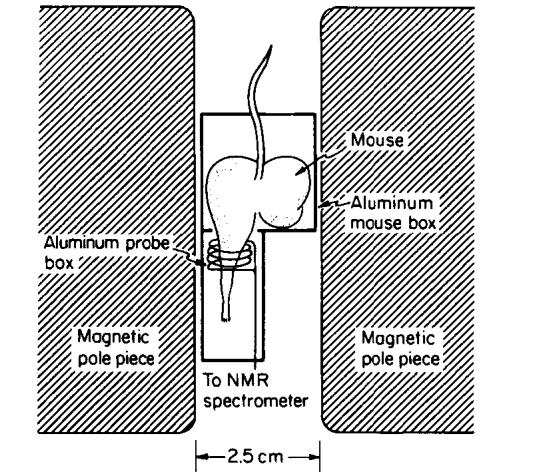
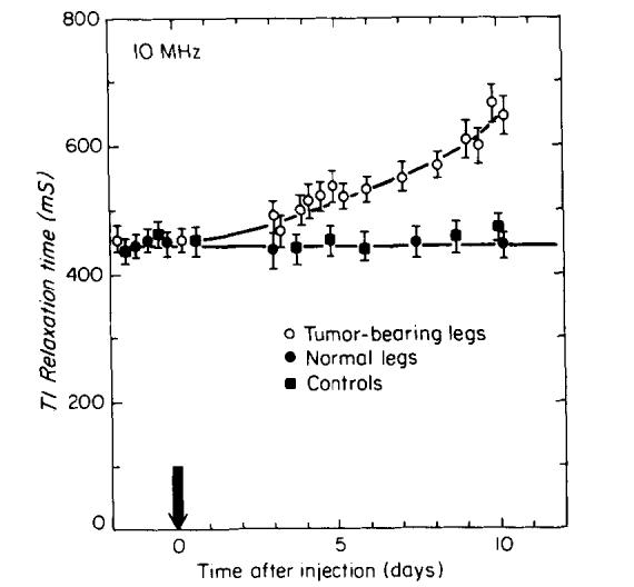
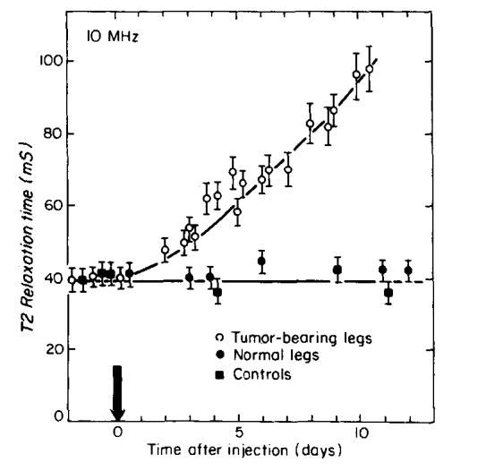
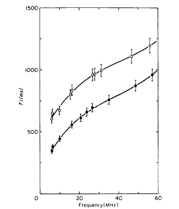
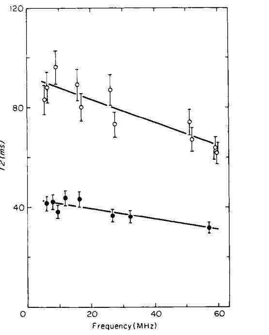
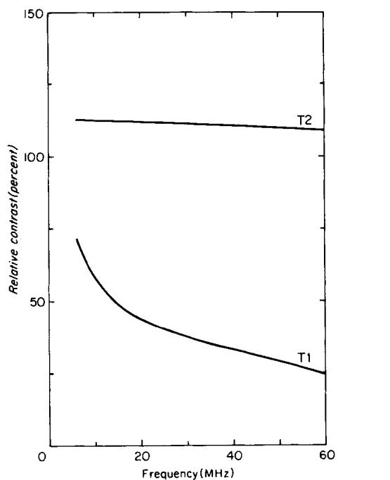
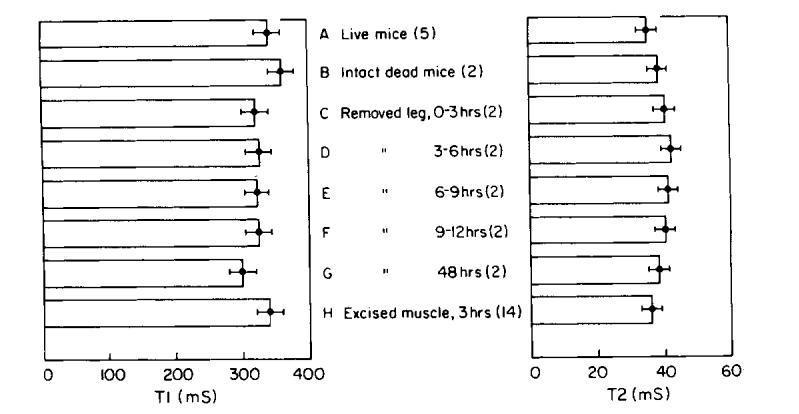
A series of solenoidal NMR probes were built to measure T1 and T2 relaxation times in vivo in the mouse, over the frequency range of 5 to 60 MHz, using inversion-recovery and spin-echo pulse sequences. KHT tumors growing in the legs of C3H mice were studied and compared with normal mouse legs. The tumor relaxation times were studied at 10 MHz during the course of tumor growth and as a function of frequency when the tumor had a mass of approximately 0.9 g. Mouse legs with tumors have higher T1 and T2 values than those without tumors over the frequency range of 5 to 60 MHz. Significant changes in both relaxation times were detected before a palpable mass could be detected. T1 contrast between normal and tumor-bearing legs decreased with increasing frequency, while T2 contrast remained nearly constant. A comparison between in vivo and in vitro measurements was done using four different types of sample preparation: live mouse, dead mouse, excised whole mouse leg, and tissue sample. These studies showed small but significant differences between the relaxation times measured in vivo and those measured in vitro.

FIG. 1

The in vivo NMR assembly, showing the mouse constrained within an aluminum box, with one leg protruding into the rf coil, and held in place with skin tape. The coil itself was contained within an aluminum box. The mouse box was kept warm with a small heating element, and the temperature was monitored with a thermistor.

FIG. 2

A response curve for a typical coil design. The data points are measured signals following a π/2 pulse from a 0.5 cm thick sample of glycerol positioned at various points along the axis of the coil. The error bars represent the standard deviation from four such measurements. The solid curve is the predicted response from Eq. [1]. The coil winding pattern is shown on the horizontal axis.

FIG. 3

Simulation of T₁ inversion-recovery experiments using an infinitely long sample extending through the mouse probe. The lower relaxation curve results when T₂ ≪ T₁ while the upper curve is for the case T₂ = T₁. Intermediate values of T₂/T₁ generate intermediate curves. The curve for T₂/T₁ = 0.1 approximates the experimental conditions when mouse legs are measured.

FIG. 4

A typical relaxation curve from an inversion-recovery experiment is shown in the upper graph. The logarithmic transformation of the data and computer fit is shown in the lower graph. The relaxation time is related to the slope of the line through the points. The data shown spans ∼3 relaxation times.

FIG. 5

T₁ of tumor-bearing legs as a function of time following injection. The time of injection is indicated by the arrow. The error bars show the estimated 5% standard deviation for T₁ measurements. The solid squares are measurements taken from the right legs of tumor-bearing mice. The solid circles are measurements taken from normal mice.

FIG. 6

T₂ of tumor-bearing legs as a function of time following injection. The time of injection is indicated by the arrow. The error bars show the estimated 7% standard deviation for T₂ measurements. The solid squares are measurements taken from the right legs of tumor-bearing mice. The solid circles are measurements taken from normal mice.

FIG. 7

T₁ vs frequency for normal and tumor-bearing legs. The open circles show T₁ for tumor-bearing legs; the solid circles for normal mice. The error bars show the estimated 5% standard deviation in the measurements. The solid curves are fits to the data using polynomials of degree three.

FIG. 8

T₂ vs frequency for normal and tumor-bearing legs. The open circles show T₂ for tumor-bearing legs; the solid circles for normal mice. The error bars show the estimated 7% standard deviation in the measurements. The solid curves are fits to the data using polynomials of degree one.

FIG. 9

Relative differences (contrast) in T₁ and T₂ between normal and tumor bearing legs, as a function of frequency; upper curve: T₂, lower curve: T₁. The curves are generated from the polynomial fits shown in Figs. 7 and 8.

FIG. 10

Results from in vivo and in vitro experiments at 6 MHz. (A) live mice; (B) intact, dead mice; (C-F) removed legs measured from death to 12 h following death, over consecutive 3 h intervals; (G) removed legs measured 48 h following death; (H) muscle tissue samples from legs, measured within 3 h after death. Error bars represent standard deviation from 25-40 experiments. Five mice were used for A, 2 mice for B-G, and 14 for H.

References

-
- BLOEMBERGEN N, PURCELL EM, POUND RV. Phys. Rev. 1948;73:679.
- HELD G, NOACK F. Z. Naturforsch. C. 1973;28:59. - PubMed
- KOENIG SH, BROWN RD, III, ADAMS D, EMERSON D, HARRISON CG. Invest. Radiol. 1984 in press. - PubMed
- ABRAGAM A. The Principles of Nuclear Magnetism. Oxford Univ. Press; (Clarendon), Oxford: 1961. pp. 82–83.
- HILL HDW, RICHARDS RE. J. Phys. E. 1968;1:977.
Publication types
MeSH terms
Grants and funding
LinkOut - more resources
Full Text Sources