. 2024 Feb 5;14(1):2894.
doi: 10.1038/s41598-024-53279-7.

Mental health and natural land cover: a global analysis based on random forest with geographical consideration

Affiliations

Mental health and natural land cover: a global analysis based on random forest with geographical consideration

Chao Li et al. Sci Rep. .

Abstract

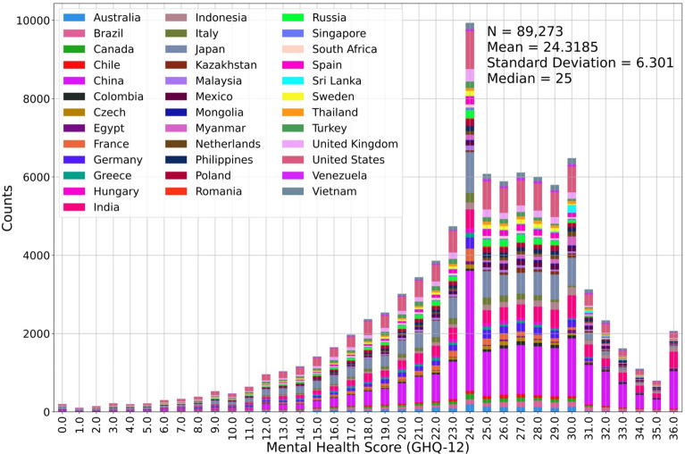
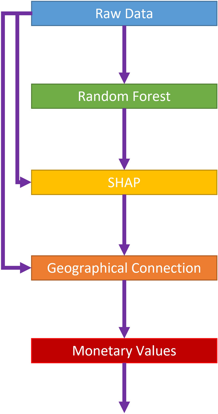
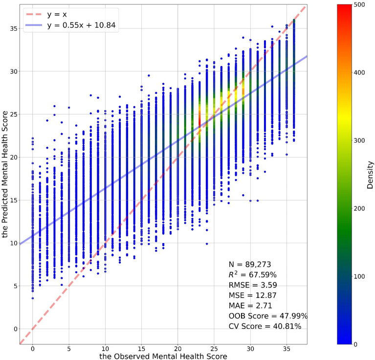
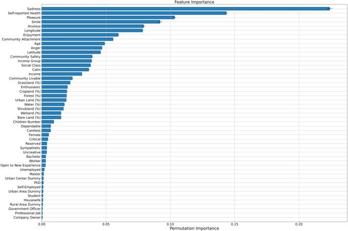
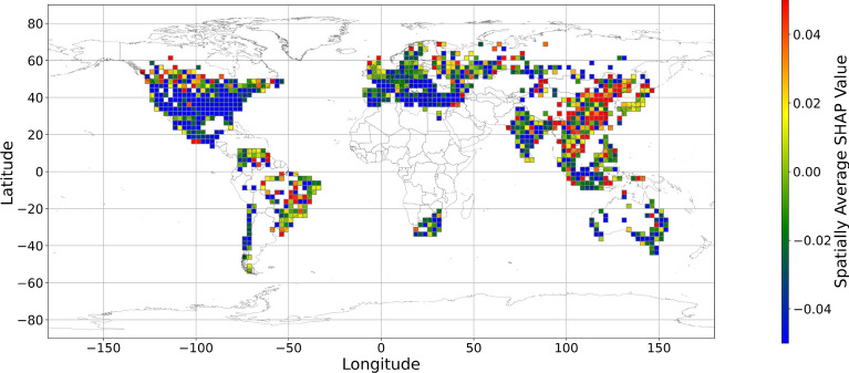
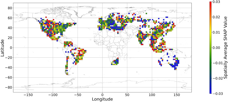
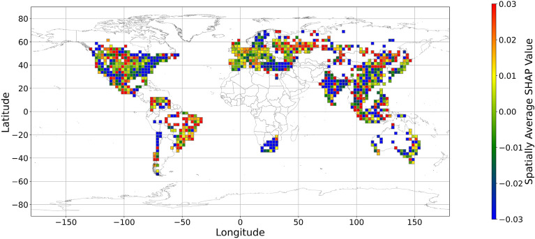
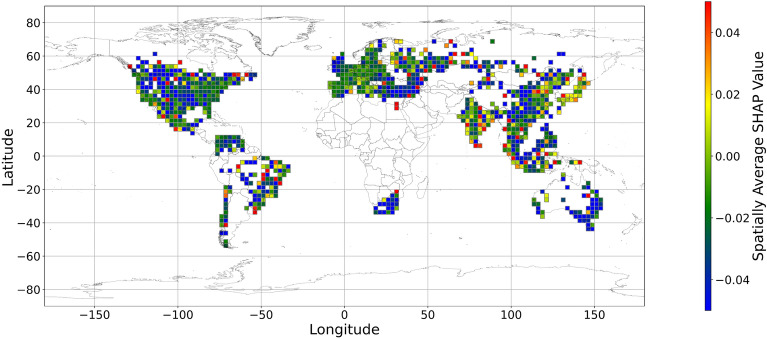
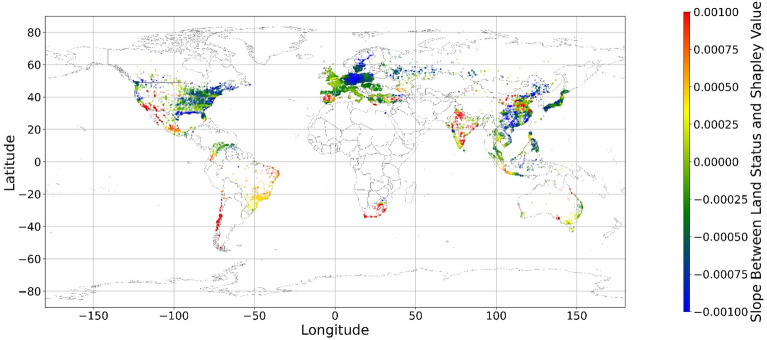
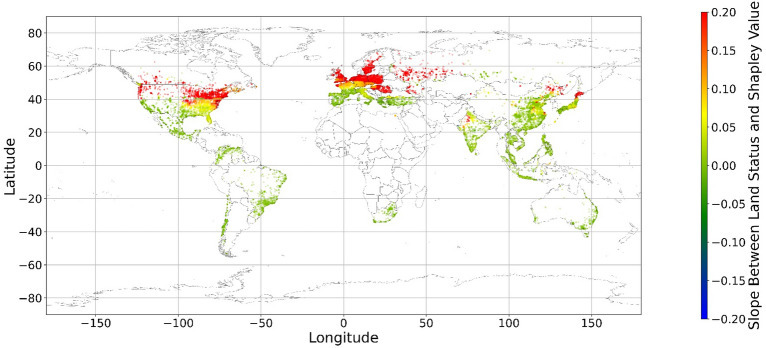
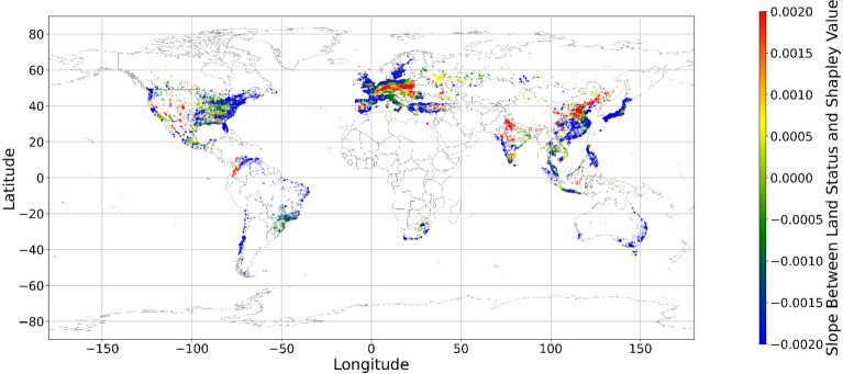
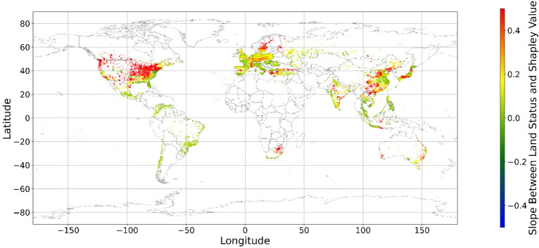
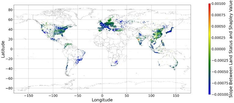
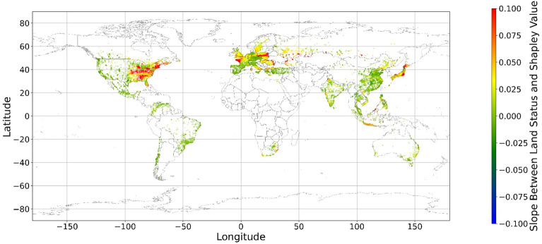
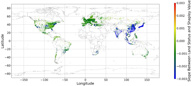
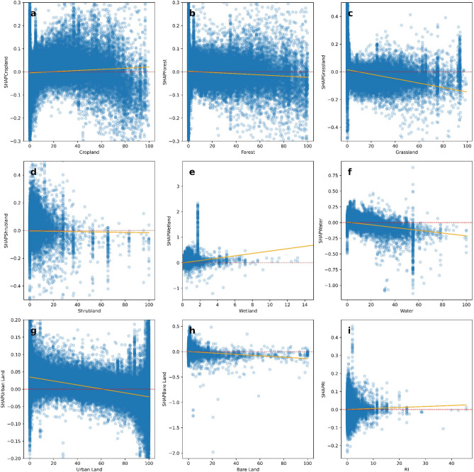
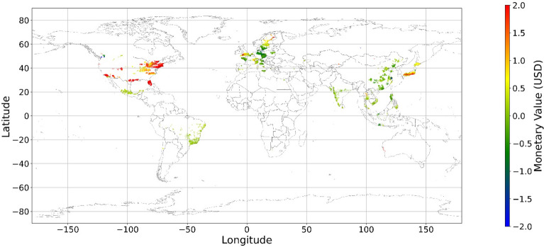
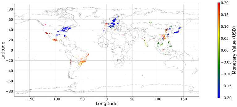
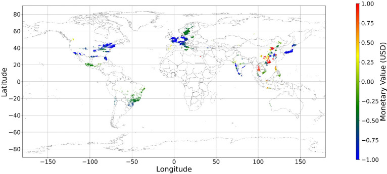
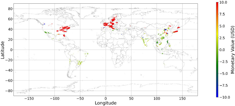
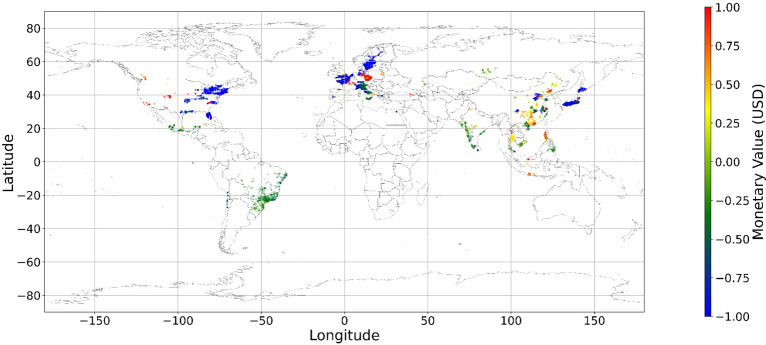
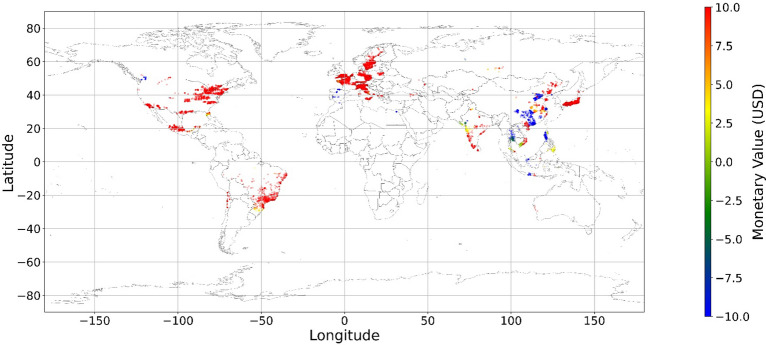
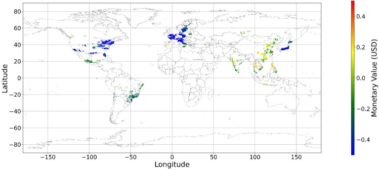
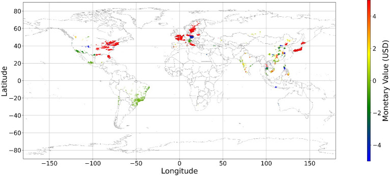
Natural features in living environments can help to reduce stress and improve mental health. Different land types have disproportionate impacts on mental health. However, the relationships between mental health and land cover are inconclusive. In this study, we aim to accurately fit the relationships, estimate the impacts of land cover change on mental health, and demonstrate the global spatial variability of impacts. In the analysis, we show the complex relationships between mental health and eight land types based on the random forest method and Shapley additive explanations. The accuracy of our model is 67.59%, while the accuracy of the models used in previous studies is usually no more than 20%. According to the analysis results, we estimate the average effects of eight land types. Due to their scarcity in living environments, shrubland, wetland, and bare land have larger impacts on mental health. Cropland, forest, and water could improve mental health in high-population-density areas. The impacts of urban land and grassland are mainly negative. The current land cover composition influences people's attitudes toward a specific land type. Our research is the first study that analyzes data with geographical information by random forest and explains the results geographically. This paper provides a novel machine learning explanation method and insights to formulate better land-use policies to improve mental health.


Conflict of interest statement

The authors declare no competing interests.

Figures

Figure 1
Figure 1
The statistical distribution of mental health assessment (the color blocks are arranged alphabetically from bottom to top according to the first letter of the country. Detailed numbers are listed in Supplementary Materials Table S1).
Figure 2
Figure 2
Analysis roadmap.
Figure 3
Figure 3
The density plots between the measured and predicted mental health score (the red dashed line is the 1:1 line. The blue line is the regression line.)
Figure 4
Figure 4
Feature importance.
Figure 5
Figure 5
The spatially average SHAP values of income. (Note: Cell size is 2.5° × 2.5°; Map’s Shapefile is downloaded from https://hub.arcgis.com/datasets/esri::world-countries-generalized/explore; We use Python 3.9.16 to plot https://www.python.org/downloads/release/python-3916/).
Figure 6
Figure 6
The spatially average SHAP values of cropland (note: Cell size is 2.5° × 2.5°; Map’s Shapefile is downloaded from https://hub.arcgis.com/datasets/esri::world-countries-generalized/explore; We use Python 3.9.16 to plot https://www.python.org/downloads/release/python-3916/).
Figure 7
Figure 7
The spatially average SHAP values of forest (Note: Cell size is 2.5° × 2.5°; Map’s Shapefile is downloaded from https://hub.arcgis.com/datasets/esri::world-countries-generalized/explore; We use Python 3.9.16 to plot https://www.python.org/downloads/release/python-3916/).
Figure 8
Figure 8
The spatially average SHAP values of grassland (Note: Cell size is 2.5° × 2.5°; Map’s Shapefile is downloaded from https://hub.arcgis.com/datasets/esri::world-countries-generalized/explore; We use Python 3.9.16 to plot https://www.python.org/downloads/release/python-3916/).
Figure 9
Figure 9
The spatially average SHAP values of shrubland (Note: Cell size is 2.5° × 2.5°; Map’s Shapefile is downloaded from https://hub.arcgis.com/datasets/esri::world-countries-generalized/explore; We use Python 3.9.16 to plot https://www.python.org/downloads/release/python-3916/).
Figure 10
Figure 10
The spatially average SHAP values of water (Note: Cell size is 2.5° × 2.5°; Map’s Shapefile is downloaded from https://hub.arcgis.com/datasets/esri::world-countries-generalized/explore; We use Python 3.9.16 to plot https://www.python.org/downloads/release/python-3916/).
Figure 11
Figure 11
The spatially average SHAP values of wetland (Note: Cell size is 2.5° × 2.5°; Map’s Shapefile is downloaded from https://hub.arcgis.com/datasets/esri::world-countries-generalized/explore; We use Python 3.9.16 to plot https://www.python.org/downloads/release/python-3916/).
Figure 12
Figure 12
The spatially average SHAP values of urban land (Note: Cell size is 2.5° × 2.5°; Map’s Shapefile is downloaded from https://hub.arcgis.com/datasets/esri::world-countries-generalized/explore; We use Python 3.9.16 to plot https://www.python.org/downloads/release/python-3916/).
Figure 13
Figure 13
The spatially average SHAP values of bare land (Note: Cell size is 2.5° × 2.5°; Map’s Shapefile is downloaded from https://hub.arcgis.com/datasets/esri::world-countries-generalized/explore; We use Python 3.9.16 to plot https://www.python.org/downloads/release/python-3916/).
Figure 14
Figure 14
The spatial scatter plot of the local coefficient between income and its SHAP value (Map’s Shapefile is downloaded from https://hub.arcgis.com/datasets/esri::world-countries-generalized/explore; We use Python 3.9.16 to plot https://www.python.org/downloads/release/python-3916/).
Figure 15
Figure 15
The spatial scatter plot of the local coefficient between cropland and its SHAP value (Map’s Shapefile is downloaded from https://hub.arcgis.com/datasets/esri::world-countries-generalized/explore; We use Python 3.9.16 to plot https://www.python.org/downloads/release/python-3916/).
Figure 16
Figure 16
The spatial scatter plot of the local coefficient between forest and its SHAP value.
Figure 17
Figure 17
The spatial scatter plot of the local coefficient between shrubland and its SHAP value (Map’s Shapefile is downloaded from https://hub.arcgis.com/datasets/esri::world-countries-generalized/explore; We use Python 3.9.16 to plot https://www.python.org/downloads/release/python-3916/).
Figure 18
Figure 18
The spatial scatter plot of the local coefficient between water and its SHAP value (map’s Shapefile is downloaded from https://hub.arcgis.com/datasets/esri::world-countries-generalized/explore; We use Python 3.9.16 to plot https://www.python.org/downloads/release/python-3916/).
Figure 19
Figure 19
The spatial scatter plot of the local coefficient between wetland and its SHAP value (map’s Shapefile is downloaded from https://hub.arcgis.com/datasets/esri::world-countries-generalized/explore; We use Python 3.9.16 to plot https://www.python.org/downloads/release/python-3916/).
Figure 20
Figure 20
The spatial scatter plot of the local coefficient between urban land and its SHAP value (map’s shapefile is downloaded from https://hub.arcgis.com/datasets/esri::world-countries-generalized/explore; We use Python 3.9.16 to plot https://www.python.org/downloads/release/python-3916/).
Figure 21
Figure 21
The spatial scatter plot of the local coefficient between bare land and its SHAP value (map’s shapefile is downloaded from https://hub.arcgis.com/datasets/esri::world-countries-generalized/explore; We use Python 3.9.16 to plot https://www.python.org/downloads/release/python-3916/).
Figure 22
Figure 22
The spatial scatter plot of the local coefficient between grassland and its SHAP value (map’s Shapefile is downloaded from https://hub.arcgis.com/datasets/esri::world-countries-generalized/explore; We use Python 3.9.16 to plot https://www.python.org/downloads/release/python-3916/).
Figure 23
Figure 23
The scatter plot between variables of interest and their SHAPs (Red dashed lines are the ablines where y-axis value equals 0; and yellow lines are linear fitting lines between x-axis value and y-axis value).
Figure 24
Figure 24
The spatial scatter plot of the monetary value of cropland (Note: Zero has been removed; Map’s Shapefile is downloaded from https://hub.arcgis.com/datasets/esri::world-countries-generalized/explore; We use Python 3.9.16 to plot https://www.python.org/downloads/release/python-3916/).
Figure 25
Figure 25
The spatial scatter plot of the monetary value of forest (Note: Zero has been removed; Map’s Shapefile is downloaded from https://hub.arcgis.com/datasets/esri::world-countries-generalized/explore; We use Python 3.9.16 to plot https://www.python.org/downloads/release/python-3916/).
Figure 26
Figure 26
The spatial scatter plot of the monetary value of grassland (Note: Zero has been removed; Map’s Shapefile is downloaded from https://hub.arcgis.com/datasets/esri::world-countries-generalized/explore; We use Python 3.9.16 to plot https://www.python.org/downloads/release/python-3916/).
Figure 27
Figure 27
The spatial scatter plot of the monetary value of shrubland (Note: Zero has been removed; Map’s Shapefile is downloaded from https://hub.arcgis.com/datasets/esri::world-countries-generalized/explore; We use Python 3.9.16 to plot https://www.python.org/downloads/release/python-3916/).
Figure 28
Figure 28
The spatial scatter plot of the monetary value of water (Note: Zero has been removed; map’s shapefile is downloaded from https://hub.arcgis.com/datasets/esri::world-countries-generalized/explore; We use Python 3.9.16 to plot https://www.python.org/downloads/release/python-3916/).
Figure 29
Figure 29
The spatial scatter plot of the monetary value of wetland (Note: Zero has been removed; map’s shapefile is downloaded from https://hub.arcgis.com/datasets/esri::world-countries-generalized/explore; We use Python 3.9.16 to plot https://www.python.org/downloads/release/python-3916/).
Figure 30
Figure 30
The spatial scatter plot of the monetary value of urban land (Note: Zero has been removed; map’s shapefile is downloaded from https://hub.arcgis.com/datasets/esri::world-countries-generalized/explore; We use Python 3.9.16 to plot https://www.python.org/downloads/release/python-3916/).
Figure 31
Figure 31
The spatial scatter plot of the monetary value of bare land (Note: Zero has been removed; map’s shapefile is downloaded from https://hub.arcgis.com/datasets/esri::world-countries-generalized/explore; We use Python 3.9.16 to plot https://www.python.org/downloads/release/python-3916/).

Similar articles

Cited by

References

    1. Diener E, Oishi S, Tay L. Advances in subjective well-being research. Nat. Hum. Behav. 2018;2:253–260. doi: 10.1038/s41562-018-0307-6. - DOI - PubMed
    1. MacKerron G, Mourato S. Happiness is greater in natural environments. Glob. Environ. Chang. 2013;23:992–1000. doi: 10.1016/j.gloenvcha.2013.03.010. - DOI
    1. Diaz S, et al. Pervasive human-driven decline of life on Earth points to the need for transformative change. Science. 2019;366:3100. doi: 10.1126/science.aax3100. - DOI - PubMed
    1. Bratman GN, et al. Nature and mental health: An ecosystem service perspective. Sci. Adv. 2019;5:0903. doi: 10.1126/sciadv.aax0903. - DOI - PMC - PubMed
    1. Malek Ž, Verburg PH. Mapping global patterns of land use decision-making. Glob. Environ. Chang. 2020;65:102170. doi: 10.1016/j.gloenvcha.2020.102170. - DOI