Climate-invariant machine learning

Abstract

Projecting climate change is a generalization problem: We extrapolate the recent past using physical models across past, present, and future climates. Current climate models require representations of processes that occur at scales smaller than model grid size, which have been the main source of model projection uncertainty. Recent machine learning (ML) algorithms hold promise to improve such process representations but tend to extrapolate poorly to climate regimes that they were not trained on. To get the best of the physical and statistical worlds, we propose a framework, termed "climate-invariant" ML, incorporating knowledge of climate processes into ML algorithms, and show that it can maintain high offline accuracy across a wide range of climate conditions and configurations in three distinct atmospheric models. Our results suggest that explicitly incorporating physical knowledge into data-driven models of Earth system processes can improve their consistency, data efficiency, and generalizability across climate regimes.

Fig. 1.. By transforming inputs x and outputs y to match their probability density functions across climates, the algorithms can learn a transformed mapping ϕ˜ that holds across climates.

To illustrate this, we show the marginal distributions of inputs and outputs in two different climates using blue and red lines, before (top) and after (bottom) the physical transformation.

Fig. 2.. Surface temperatures in the three used atmospheric models.

Prescribed surface temperature (in kelvin) for (left) the aquaplanet SPCAM3 model and (right) the hypohydrostatic SAM model. (Center) Annual-mean, near-surface air temperatures in the Earth-like SPCESM2 model.

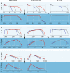
Fig. 3.. Physical transformations can align distributions across climates.

We show the univariate distributions of selected raw inputs x: (A) 600-hPa specific humidity; (B) 850-hPa temperature; and (C) latent heat flux (LHF) in the cold (blue), reference (gray), and warm (red) simulations of each model (SPCAM3, SPCESM2, and SAM). For each variable, we also show the PDFs of the transformed inputs $\tilde{\mathit{x}}$ as discussed in the Theory section. From top to bottom, the variables are q (grams per kilogram), relative humidity (RH), T (kelvin), B_plume (meters per square second), LHF (watts per square meter), and LHF_Δq (kilograms per square meter per second). For a given variable and transformation, we use the same vertical logarithmic scale across models.

Fig. 4.. All neural networks (NNs), trained in the cold climate, exhibit low error in the cold climate’s test set, but much larger error in the warm climate’s test set.

(A) Low error in the cold climate’s test set. (B) Larger error in the warm climate’s test set. This generalization error decreases as inputs are incrementally transformed: first no transformation (blue), then the vertical profile of specific humidity (orange), then the vertical profile of temperature (green), and lastly LHFs (red). For reference, the purple line depicts an NN trained in the warm climate. We depict the tendencies’ mean-squared error (MSE) versus pressure, horizontally averaged over the tropics of SPCAM3 aquaplanet simulations, for the four model outputs: total moistening ( $\dot{q}$ ), total heating ( $\dot{T}$ ), longwave heating (lw), and shortwave heating (sw). Given that the raw-data NN’s generalization error (blue line) greatly exceeds that of the transformed NNs, we zoom in on each panel to facilitate visualization.

Fig. 5.. Model error across temperatures and configurations.

MSE (in W² m⁻⁴) of six models trained in three simulations (first column) and evaluated over the training or validation set of the same and two other simulations (last four columns). The models (second column) are raw-data (RD) or climate-invariant (CI), and MLRs or neural nets (NN), and sometimes include DP layers preceded by a BN layer (DN). The models are trained for 20 epochs. We first provide the MSE corresponding to the epoch of minimal validation loss, then the MSE averaged over the five epochs with lowest validation losses (in parentheses), and lastly the MSE divided by the baseline MSE, where we use the raw-data MLR as baseline. Note that “different temperature” refers to (+4 K) for (−4 K) training sets and vice versa. In each application case, we highlight the best model’s error using bold font.

Fig. 6.. Climate-invariant NNs address the raw-data NNs’ generalization problems in the warm tropics.

This is demonstrated by the 500-hPa subgrid heating’s coefficient of determination R₂ calculated over the test set for the raw-data (A) and climate-invariant (B) NNs. We train NNs using the cold (−4 K) training set of each model (SPCAM3, SPCESM2, and SAM). We note that these NNs do not use DP nor BN, and we refer the readers to fig. S8 for latitude-pressure cross sections.

Fig. 7.. Explainable artificial intelligence suggests that climate-invariant mappings are more spatially local.

We depict ℳ for the (A) raw-data and (B) climate-invariant NNs trained in the SPCAM3 (+4 K) warm aquaplanet simulation. The x axes indicate the inputs’ vertical levels, from the surface (left, 10³ hPa) to the top of the atmosphere (right, 0 hPa), while the y axes indicate the outputs’ vertical levels, from the surface (bottom, 10³ hPa) to the top of the atmosphere (top, 0 hPa). We additionally indicate the 200-hPa vertical level with black dashed lines.

Fig. 8.. Climate-invariant (CI) NNs trained on datasets containing both cold (−4 K) and warm (+4 K) samples outperform raw-data (RD) models offline in ≈95% of cases, with less sensitivity to the data partition used for training.

Dots on the left represent the median RD error from a 10-fold cross-validation without replacement, with horizontal ticks indicating the first and ninth deciles. Stars on the right correspond to the median CI error. Ticks denote the majority of cases, for which CI models outperform RD models, even when data from both climates are available; crosses indicate the rare exceptions. We use a logarithmic scale for both axes.

Fig. 9.. Proposed five-step workflow to find climate-invariant transformations.

The transformations help ML models generalize from a reference (ref.) climate to a target one, using (top) a baseline MLR as an initial guide.

References

1. Reichstein M., Camps-Valls G., Stevens B., Jung M., Denzler J., Carvalhais N., Prabhat, Deep learning and process understanding for data-driven Earth system science. Nature 566, 195–204 (2019). - PubMed
1. T. Beucler, I. Ebert-Uphoff, S. Rasp, M. Pritchard, P. Gentine, “Machine learning for clouds and climate” in Clouds and their Climatic Impacts: Radiation, Circulation, and Precipitation (John Wiley & Sons, 2023), pp. 325–345.
1. Irrgang C., Boers N., Sonnewald M., Barnes E. A., Kadow C., Staneva J., Saynisch-Wagner J., Towards neural Earth system modelling by integrating artificial intelligence in Earth system science. Nat. Mach. Intell. 3, 667–674 (2021).
1. de Burgh-Day C. O., Leeuwenburg T., Machine learning for numerical weather and climate modelling: A review. Geosci. Model Dev. 16, 6433–6477 (2023).
1. Molina M. J., O’Brien T. A., Anderson G., Ashfaq M., Bennett K. E., Collins W. D., Dagon K., Restrepo J. M., Ullrich P. A., A review of recent and emerging machine learning applications for climate variability and weather phenomena. Artif. Intell. Earth Syst. 2, 220086 (2023).