Converting an allocentric goal into an egocentric steering signal

Abstract

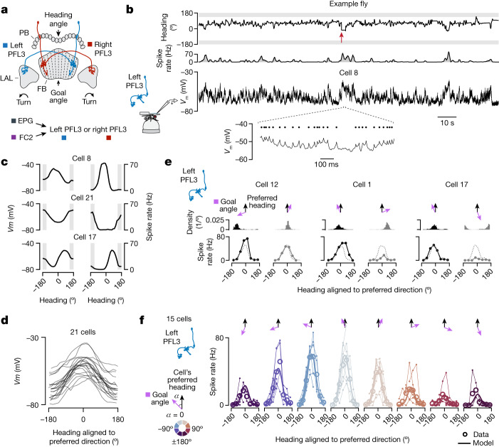
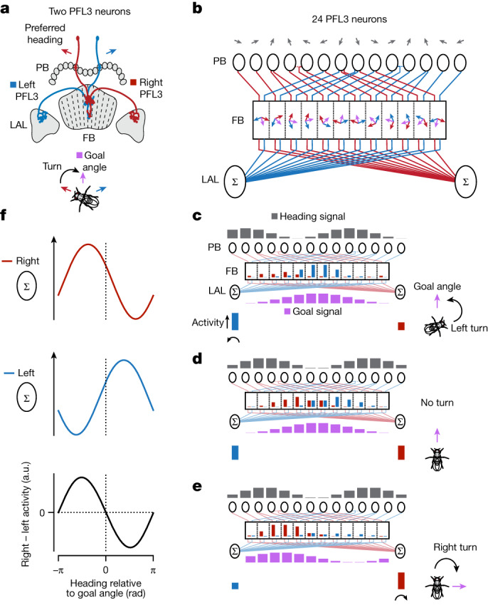
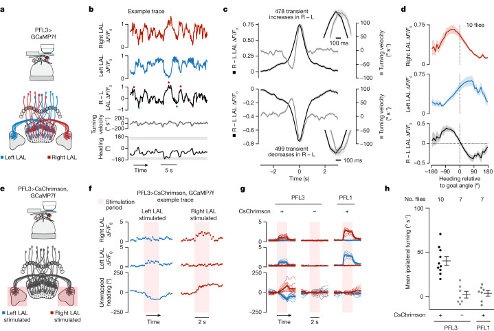
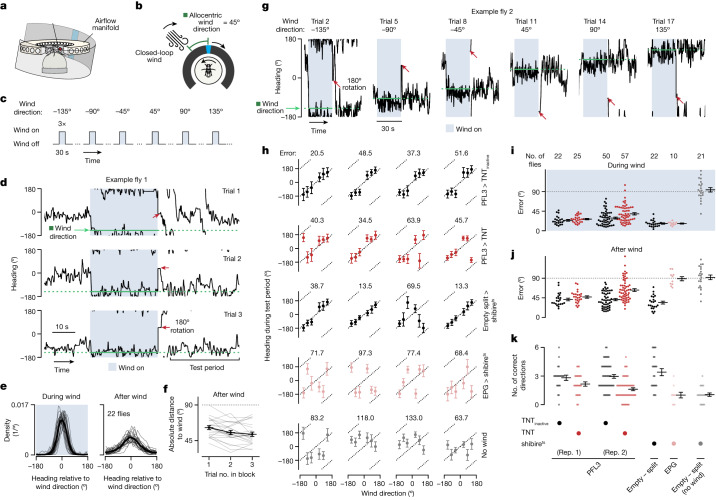
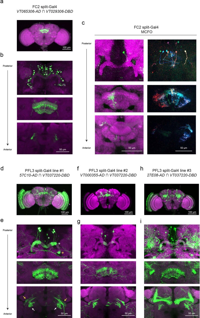
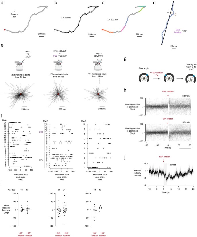
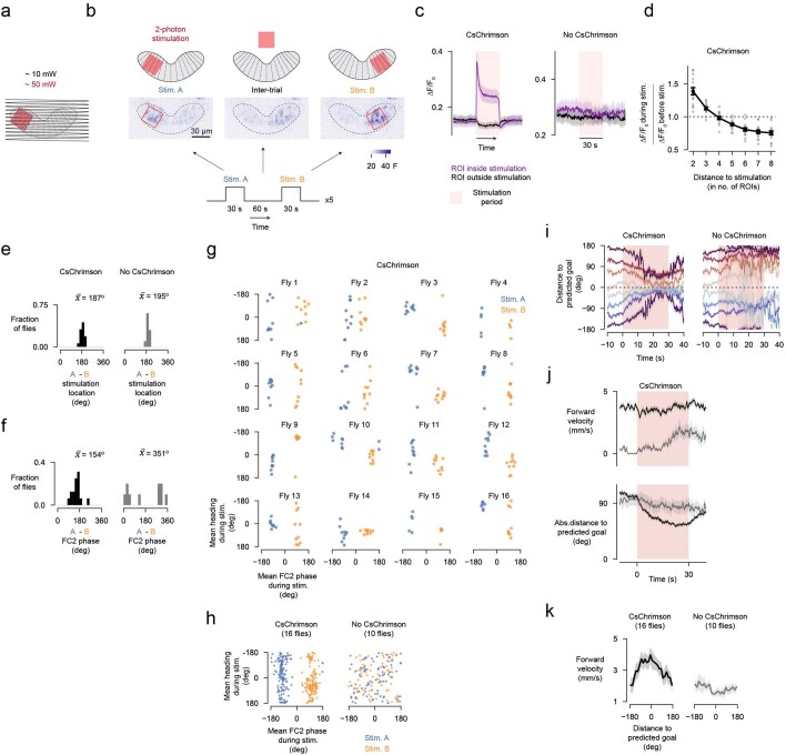
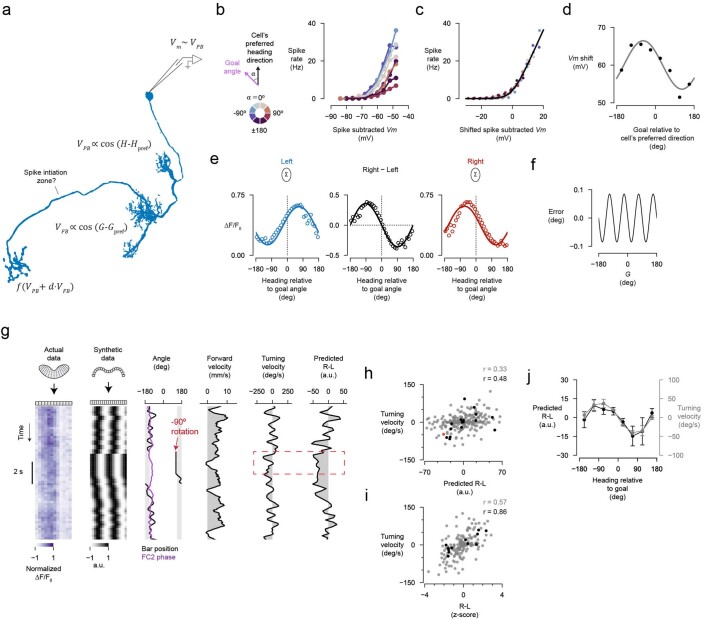
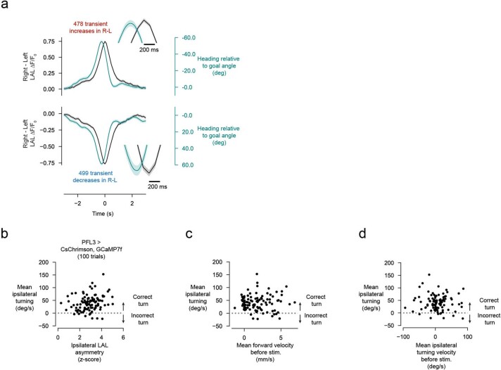
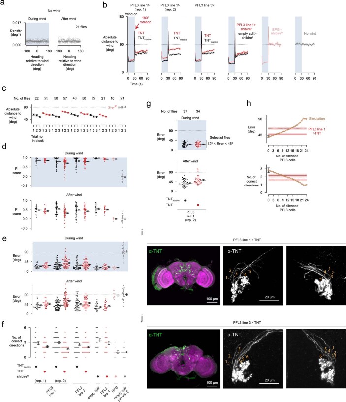
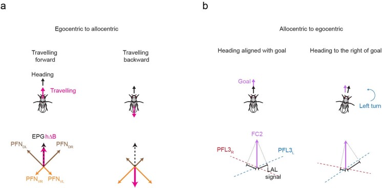
Neuronal signals that are relevant for spatial navigation have been described in many species^1-10. However, a circuit-level understanding of how such signals interact to guide navigational behaviour is lacking. Here we characterize a neuronal circuit in the Drosophila central complex that compares internally generated estimates of the heading and goal angles of the fly-both of which are encoded in world-centred (allocentric) coordinates-to generate a body-centred (egocentric) steering signal. Past work has suggested that the activity of EPG neurons represents the fly's moment-to-moment angular orientation, or heading angle, during navigation^2,11. An animal's moment-to-moment heading angle, however, is not always aligned with its goal angle-that is, the allocentric direction in which it wishes to progress forward. We describe FC2 cells¹², a second set of neurons in the Drosophila brain with activity that correlates with the fly's goal angle. Focal optogenetic activation of FC2 neurons induces flies to orient along experimenter-defined directions as they walk forward. EPG and FC2 neurons connect monosynaptically to a third neuronal class, PFL3 cells^12,13. We found that individual PFL3 cells show conjunctive, spike-rate tuning to both the heading angle and the goal angle during goal-directed navigation. Informed by the anatomy and physiology of these three cell classes, we develop a model that explains how this circuit compares allocentric heading and goal angles to build an egocentric steering signal in the PFL3 output terminals. Quantitative analyses and optogenetic manipulations of PFL3 activity support the model. Finally, using a new navigational memory task, we show that flies expressing disruptors of synaptic transmission in subsets of PFL3 cells have a reduced ability to orient along arbitrary goal directions, with an effect size in quantitative accordance with the prediction of our model. The biological circuit described here reveals how two population-level allocentric signals are compared in the brain to produce an egocentric output signal that is appropriate for motor control.

Fig. 1. FC2 neurons express a stable activity bump in the fan-shaped body during virtual rotations of the fly.

a, Comparing heading angle (grey) and goal angle (purple) to drive turning. b, Schematic of three central-complex structures and the LALs of the fly brain. c,d, Schematics of EPG neurons (c) and FC2 neurons (d). e, Virtual reality setup for recording neural activity in a walking fly. f, Virtual 2D trajectory from a single fly performing menotaxis from which we simultaneously recorded GCaMP activity (26-min recording). An algorithmically detected menotaxis bout is highlighted in black (Methods). Red dot marks the start of the trajectory. g, Trajectories of all menotaxis bouts from the EPG and FC2 imaging datasets. Trajectories were aligned to begin at the same location (red dot). h, Example trace of jGCaMP7f activity of EPG neurons in the protocerebral bridge (PB). Left, EPG ΔF/F₀ over time. Middle, bar position (that is, the inverse of the fly’s heading angle) (black) and the EPG phase estimate (grey). Shaded area represents the 90° gap where the bar is not visible. Right, forward walking velocity. The top trace shows a time period during which the fly meandered rather than performing menotaxis. The bottom trace shows a later moment, when the same fly maintained a relatively consistent heading angle. i, Example trace of jGCaMP7f activity of FC2 neurons in the fan-shaped body (FB) (viewed dorsally). j, Experimental paradigm for dissociating heading and goal signals. k,l, Example EPG (k) and FC2 (l) traces during +90° virtual rotations (red arrow). m, Individual ±90° rotation trials (downward red arrows indicate 90° rotation). Top, bar position zeroed at onset of rotation. Bottom, EPG phase zeroed at onset of rotation; thick lines show the mean across flies. Fourteen ±90° trials from 5 flies are shown. See Methods for trial selection criteria. Shaded area marks the 2 s period when the bar was kept stable, at a ± 90° offset, before giving the fly closed-loop control. n, Same as m but for seventeen ±90° rotation trials from 7 FC2 flies. o, Mean phase value during the final 1 s of the open-loop period in m,n. Each dot is the mean for one fly. Horizontal lines depict mean ± s.e.m. across flies. Dashed line shows the expected phase position if the position in the brain of a bump were to track the bar angle. V-test for EPG flies: μ = 90°, P = 7.99 × 10⁻³. V-test for FC2 flies: μ = 0°, P = 6.65 × 10⁻⁴. Source Data

Fig. 2. Stimulating FC2 neurons in a contiguous subset of fan-shaped body columns induces flies to orient along defined goal angles.

a, Simultaneous imaging and focal stimulation of FC2 neurons. b, Stimulation protocol. Images show average z-projection of raw fluorescence signal during the stimulation period from a single trial. Red squares mark the two locations of two-photon (2p) stimulation in the fan-shaped body (referred to as stim. A and stim. B). a.u., arbitrary units. Scale bar (middle left), 30 µm. c, Example FC2 ΔF/F₀ signal and behavioural traces during a CsChrimson experiment. Left, FC2 activity over time. The red heat map shows the fraction of pixels of each column’s region of interest (ROI) that is inside the stimulation (stim.) ROI. Right, heading direction of a fly over time. Shaded blue and orange areas indicate the stimulation period. Bottom, probability distribution of the fly’s heading direction across all trials for each stimulation location. d, Same as c but for a control fly that did not express CsChrimson. e, Probability distributions of heading direction for 10 (out of the 16 total) CsChrimson-expressing flies (left) and 10 (out of 10) control flies that did not express CsChrimson (right). The heading direction was zeroed by subtracting the fly’s mean heading direction across all stim. A trials. f, Mean probability distributions for all flies. g, Difference between mean heading direction during stim. A and stim. B trials for each fly (black dots). Mean ± s.e.m. across flies is indicated. Dashed red line indicates the expected difference in heading direction based on the mean difference in the stimulation location for each group (see Extended Data Fig. 4e). V-test for CsChrimson flies: μ = −173.4° (left dashed line), P = 1.49 × 10⁻³. V-test for no CsChrimon flies: μ = −164.9° (right dashed line), P = 0.93. Source Data

Fig. 3. PFL3 neurons show conjunctive spike-rate tuning to heading and goal angles.

a, Two schematic PFL3 neurons. b, PFL3 patch-clamp data from a fly performing menotaxis. Top, the fly’s heading relative to the bar (0° indicates bar in front). Red arrow shows a 90° bar jump. Second row, spike rate. Third row, membrane potential (V_m). Bottom, magnified view of V_m. Black dots indicate spikes. c, Left, V_m (with spikes removed) tuning curves to heading for three example PFL3 cells. Right, spike-rate tuning curves. d, V_m (spikes removed) tuning curves for all PFL3 neurons, aligned to each cell’s preferred heading direction. e, Tuning curves for three example left PFL3 neurons binned according to the angular difference between the fly’s goal angle and the cell’s preferred heading direction. Note larger tuning-curve amplitudes when the fly’s goal is to the left of the cell’s preferred direction (black) compared to when it is to the right (grey). Dashed line, tuning curve using data from the entire recording. Top, histogram of behavioural heading angles (aligned to the cell’s preferred direction) in association with the spike-rate tuning curves (bottom). f, Population-averaged, spike-rate tuning curves to heading, parsed by the flies’ goal angle. Each column represents a different bin of goal angles relative to the cell’s preferred direction. Thin lines and small open circles represent individual cell tuning curves. Data are missing in portions of the x axis for individual cells because a fly does not always experience the full range of heading directions for each goal direction, even with bar jumps. Large open circles represent mean across cells. Thick lines show the model fit (Methods). Source Data

Fig. 4. Model for how PFL3 neurons compare heading and goal angles to generate a steering signal.

a, Schematic of two PFL3 neurons with offset preferred heading directions (red and blue arrows). The two cells project to a common column in the fan-shaped body. These two PFL3 cells could lead a fly to stabilize an allocentric goal angle midway between their preferred heading angles (purple arrow). b, Wiring diagram of all 24 PFL3 neurons in the fly brain. Each grey arrow represents the preferred heading angle that a PFL3 neuron innervating a given glomerulus of the protocerebral bridge is expected to inherit from presynaptic heading-sensitive EPG and ∆7 neurons in that glomerulus (Extended Data Fig. 5a–g). Blue and red arrows represent the bridge-inherited, preferred heading angle H_pref of the left and right PFL3 neurons that innervate a given column in the fan-shaped body. Purple arrows represent each column’s preferred goal angle G_pref. c, Example heading and goal input bumps to the PFL3 population and the predicted output signal from individual PFL3 neurons and the PFL3 population. The neural signals in the schematic apply to the situation depicted by the fly on the right. Dark grey bar plots show the spatial activity pattern of the heading inputs to PFL3 cells in the bridge. The height of each bar is proportional to the cosine of the angle between the direction of the fly’s heading and the corresponding (grey) preferred heading arrow in b. Purple bar plots show the spatial activity pattern of goal (FC2) inputs to PFL3 cells in the fan-shaped body. The height of each bar is proportional to the cosine of the difference between the fly’s goal angle and the corresponding (purple) preferred goal angle of each column in b. Red and blue bar plots in the fan-shaped body represent the activity of individual PFL3 neurons, determined by a nonlinear function of their summed protocerebral bridge and fan-shaped body inputs. Red and blue bar plots below the sigma symbol indicate summed activity for left and right PFL3 neurons in the LAL. d,e, Same as c but for different heading and goal angles. f, Model-predicted, population-level activity in the right and left LAL (red and blue curves) and predicted turning signal (right-minus-left LAL activity, black curve).

Fig. 5. Imaging and perturbing PFL3 activity in the LALs supports the model.

a, Two-photon calcium imaging of the LAL of flies expressing jGCaMP7f in PFL3 neurons labelled by split-Gal4 line 57C10-AD ∩ VT037220-DBD. b, Example time series of GCaMP imaging data. In the third row, red dots mark transient increases in the LAL right – left (R − L) ΔF/F₀ signal and blue dots mark transient decreases. c, The flies’ turning velocity (grey) and R – L signal (black) aligned to transient increases (top) or decreases (bottom) in the R − L signal. Insets show that the peak in the R − L asymmetry precedes the peak in turning velocity by around 100 ms. Mean ± s.e.m. across transients is shown (from ten flies). d, LAL activity plotted as a function of the fly’s heading relative to its goal angle. Mean ± s.e.m. across flies is shown. e, Stimulation of PFL3 cells in either left or right LAL while simultaneously performing calcium imaging from the same cells. We used flies that co-expressed CsChrimson and jGCaMP7f in PFL3 neurons labelled by split-Gal4 line VT000355-AD ∩ VT037220-DBD. f, Left, example trial in which we stimulated the left LAL. Bottom row, unwrapped heading zeroed at onset of stimulation. A decrease in the unwrapped heading signal means the fly turned left. Right, example trial with the right LAL stimulated. g, Fly-averaged GCaMP and turn signals (thin lines) for left (blue) and right (red) LAL stimulation of PFL3 or PFL1 cells. The thick line shows the average across flies. h, Mean ipsilateral (relative to the stimulation side) turning velocity during the 2-s stimulation period. Dots show the mean for individual flies and the mean ± s.e.m. across flies is indicated. PFL3 CsChrimson flies have a greater ipsilateral turning velocity than non CsChrimson PFL3 flies (P = 1.93 × 10⁻⁵, Welch’s two-sided t-test). PFL1 Chrimson flies show no significant change ipsilateral turning velocity relative to controls (P = 0.76, Welch’s two-sided t-test). Source Data

Fig. 6. Flies expressing a synaptic blocker in subsets of PFL3 cells have a reduced ability to navigate along remembered goal directions in a wind-induced angular memory task.

a, Setup for delivering airflow and visual stimuli in closed loop. A circular manifold of 36 equally spaced tubes delivers airflow to the head-fixed fly from different directions. b, To simulate the experience of a fixed allocentric wind direction, the airflow angle changed in rotational closed loop with the flies’ turns on the ball. The airflow angle had a fixed angular offset to the bar, which also rotated in closed loop. c, Task structure. d, Heading over time for the first three trials in a control fly (empty split-Gal4>shibire^ts). The upwind heading is indicated by the green dotted line. Red arrows indicate 180° virtual rotations of the fly (bar jumps) after the airflow is turned off. e, Heading relative to wind distributions from control flies (empty split-Gal4>shibire^ts) when the wind is on (left) and when the wind is off, during the test period (right). Thin lines represent individual flies. The thick line shows the mean across flies. f, Mean absolute distance between heading and wind angles during the test period as a function of the trial number within a block. Grey lines, mean of individual control flies (empty split-Gal4>shibire^ts). Black line shows mean ± s.e.m across flies (n = 22). g, Second trial of each wind-direction block from an example control fly (empty split-Gal4>shibire^ts). Red arrows indicate 180° rotation. h, Top row, mean heading direction during the test period versus the wind direction for four example control flies (PFL3>TNT_inactive). TNT_inactive denotes expression of a mutationally inactive TNT. Each dot represents the fly’s mean heading in the second and third trials of each wind-direction block. We refer to the absolute difference between this value and the wind direction as the wind-direction error (error). For each fly, the mean error across all six wind directions is indicated above each plot. Data shown as mean ± s.d. in heading across the second and third trials of each block. Bottom four rows show example flies for each of the following genotypes: PFL3>TNT, empty split-Gal4>shibire^ts, EPG>shibire^ts, and empty split-Gal4>shibire^ts flies for which the airflow was turned off. i, Error during the wind period for each group. For PFL3>TNT and PFL3>TNT_inactive groups, we ran two independent replicates, shown separately. Each dot shows the mean for a fly across all wind directions. Mean ± s.e.m. across flies is indicated for each genotype. j, Same as i but for the test period. PFL3>TNT flies exhibited a greater error than PFL3>TNT_inactive flies (P = 0.05 for replicate (rep.) 1 and P = 1.20 × 10⁻⁶ for replicate 2, two-sided Mann–Whitney U-test; combined P value = 1.08 × 10⁻⁶, Fisher’s method). k, Number of wind directions that each fly correctly oriented along. Each dot represents one fly. Mean ± s.e.m. across flies is indicated. PFL3>TNT flies oriented along fewer correct directions than PFL3>TNT_inactive flies (P = 0.04 for replicate 1 and P = 5.25 × 10⁻⁷ for replicate 2, two-sided Mann–Whitney U-test; combined P value = 3.90 × 10⁻⁷, Fisher’s method). PFL3 data are from the 57C10-AD ∩ VT0372202-DBD split-Gal4 line (PFL3 line 1). Source Data

Extended Data Fig. 1. FC2 and PFL3 split-Gal4 lines characterization.

a, Whole-brain GFP expression driven by the split-Gal4 line VT065306-AD ∩ VT029306-DBD (green), which labels FC2 neurons, and anti-Bruchpilot neuropil stain (magenta). b, Each panel shows a maximum z-projection at a different depth of the anterior-posterior axis. Top: The number of GFP positive somas, roughly 70 to 100, is comparable to the 88 FC2 neurons identified in the hemibrain. Middle: fan-shaped body. Bottom: crepine. Each FC2 neuron projects unilaterally to the crepine, a symmetric structure that flanks the central complex and is situated dorsal to the lateral accessory lobes. c, Multicolor flip-out of a single FC2 neuron (left) and several FC2 neurons (right) labeled by VT065306-AD ∩ VT029306-DBD. The innervation pattern in the fan-shaped body is consistent with the FC2B or FC2C subtypes. While the GFP expression in this line suggests that it is selective for crepine projecting neurons with FC2-like anatomy, it is possible that there are some non-FC2 central complex neurons labeled by the line as well. d, Whole-brain GFP expression in the 57C10-AD ∩ VT037220-DBD split-Gal4 line (used for LAL imaging and silencing experiments), which labels PFL3 neurons. e, Top: protocerebral bridge. The white asterisk highlights a glomerulus lacking clear PFL3 signal, indicating that the line does not target all 24 PFL3 cells. The yellow asterisk shows a glomerulus innervated by a non-PFL3 neuron (likely a PEG neuron), since PFL3 neurons do not innervate the outer two glomeruli in the bridge. Middle: fan-shaped body. Bottom: lateral accessory lobes. White arrows highlight PFL3 expression in the left and right LAL. Yellow arrows mark non-PFL3 expression, which we excluded from our regions of interest for imaging analysis. f-g, Same as panels d-e but for VT000355-AD ∩ VT037220-DBD split-Gal4 line (used for patch-clamp and LAL-stimulation experiments). This line also stochastically labels PEG neurons. This was not a concern for either our patch-clamp (see Extended Data Fig. 6) or our LAL-stimulation experiments, since PEG neurons do not innervate the LAL. h-i, Same as panels d-e but for 27E08-AD ∩ VT037220-DBD split-Gal4 line (used for silencing experiments). Whereas this line drives significant GFP expression outside the central complex, including in the mushroom body (panel i, bottom), TNT expression driven by this same line appeared to be sparse outside the central complex (see Extended Data Fig. 11j). Source Data

Extended Data Fig. 2. Using the fly’s virtual 2D trajectory to analyze menotaxis behaviour; and following a virtual rotation, flies slow down and turn so as to return to their previous heading.

a, Example virtual 2D trajectory of a fly performing menotaxis (during a PFL3 patch-clamp recording). Red dot marks the start of the trajectory. b, Ramer-Douglas-Peucker algorithm reduces the number of x,y coordinates in the trajectory using the parameter ξ, the maximum allowed distance between the simplified and original trajectories. Black dots show the simplified coordinates. c, The fly’s displacement between each x,y point of the simplified trajectory, L, is computed. Segments of the fly’s trajectory where L > 200 mm were considered “menotaxis bouts” and thus further analyzed (colored portions of the trajectory). d, An example menotaxis bout from the trajectory in panel c. The fly’s goal angle is defined as the fly’s mean heading direction during the bout, excluding timepoints when the fly is standing still. e, All menotaxis bouts from flies used in this paper. First column: PFL3 patch-clamp dataset (related to Fig. 3). Middle column: EPG and FC2 imaging dataset (related to Fig. 1). Third column: PFL3 LAL imaging dataset (related to Fig. 5d). f, Goal angles for each menotaxis bout for each fly for datasets shown in panel e. g, To assess whether a fly was actively maintaining its heading direction, we virtually rotated the fly by discontinuously jumping the bar ±90° from its position immediately before the jump. The bar remained static at its new position for 2 s and then the fly regained closed-loop control. h, The fly’s heading relative to its goal angle for ±90° rotation trials from our PFL3 patch-clamp dataset. Only trials where the circular standard deviation of the fly’s heading direction during the 60 s prior to the bar jump was less than 45° (excluding timepoints when the fly was standing still) were analyzed here (55-74% of all trials were analyzed depending on the dataset). For this analysis, we defined the fly’s goal angle as its mean heading in the 60 s before the bar jump, excluding timepoints in which the fly was standing still. i, Mean heading relative to the fly’s goal angle during the 30 to 60 s after the bar jump for trials from each dataset shown in panels e-f. Each dot is the mean for an individual fly. Horizontal lines show mean ± s.e.m. across flies. j, Mean forward walking velocity around the time of bar jumps for trials shown in panel h. Shaded area marks the 2 s when the bar remained static. Mean ± s.e.m. across flies is shown. Source Data

Extended Data Fig. 3. Relationship between FC2 activity and fly behaviour.

a, Correlation between EPG phase or FC2 phase and fly heading. Each dot represents one fly. Mean ± s.e.m. across flies is indicated. b, Cross-correlation between phase velocity and behavioural turning velocity. FC2 data are in purple and EPG data are in grey. A positive lag means that a change in heading precedes a change in the neuronal signal. Mean ± s.e.m. across flies is shown. c, Individual ±90° rotation trials for 113 trials from 9 flies in which we imaged EPG neurons. In contrast to Fig. 1, here we did not require for a trial to occur within a menotaxis bout (see Methods) or require that the fly return within 45° from its heading before the bar jump. Thick lines show the mean across flies. d, Same as panel c but for 140 trials from 15 flies in which we imaged FC2 neurons. Note that, on average, the FC2 phase slowly drifts away from its initial position. This small drift may be due to trials where the fly’s goal angle genuinely drifted to the fly’s new heading angle after the bar jump, which seems plausible given that on many trials analyzed here the fly did not turn so as to reorient themselves along their previous heading. e, Mean phase value during final 1 s of the open-loop period in panels c and d. Each dot is the mean for one fly. Horizontal lines show the mean ± s.e.m. across flies. V-test for EPG flies: μ = 90°, p = 2.49 × 10⁻⁵. V-test for FC2 flies: μ = 0°, p = 7.69 × 10⁻⁸. f, Example trace showing an abrupt change in the position of the FC2 bump in the fan-shaped body. g, Left: Each thin line shows an algorithmically-detected rapid change in the FC2 phase position, zeroed to the onset of the change in phase. Right: bar position, zeroed to the onset of the change in phase, during these moments. Thick lines show the mean across 141 transients from 15 flies. That the FC2 phase has the capacity to move by more than 90° within less than 2 s (the magnitude and duration of our bar jumps) suggests that the stability of the FC2 phase during virtual rotations was not due to the FC2 phase simply reflecting a low-pass filtered estimate of the fly’s heading. h, Left: example FC2 ΔF/F₀ signal and behavioural traces from a fly that occasionally deviated from its goal angle. The teal arrow marks a moment when the FC2 phase did not remain stable, but the fly nonetheless returned to its putative goal direction. One interpretation of the moment marked in teal is that inputs other than the longer-term menotaxis goal input to the FC2 system briefly dominated, which led the FC2 phase to drift. However, once the fly re-entered a menotaxis behavioural state and wished to progress forward, the FC2 phase locked back in to the menotaxis angle, communicating it to the PFL3 population to guide steering. In this view, the fan-shaped body may encode multiple potential goals, with the actual goal chosen from this set in a state-dependent manner and the FC2 calcium signal might be best viewed as a conduit between these long-term navigational goals and the central-complex’s pre-motor output. The red arrow marks an occasion when the FC2 phase remained stable throughout a brief deviation in heading direction. Right: expanded view of time period marked by teal box and red box. i, Example FC2 ΔF/F₀ signal and behavioural traces from a fly that was rotating in time and not stabilizing a consistent heading direction. This trace highlights that the FC2 phase can be well-estimated during moments where our algorithm would not detect that the fly is performing menotaxis. j, FC2 activity across the fan-shaped body from a single timeframe. k, Schematic of how we computed the population vector average (PVA) strength from FC2 activity. Each fan-shaped body column region-of-interest (ROI) is treated as a vector (thin arrows). The angle of each vector is determined by the position of the column in the fan-shaped body and the length of the vector is determined using the ΔF/F₀ value. The PVA strength is the length of the resulting mean vector (thick arrow). l, Difference between the mean ΔF/F₀ two seconds before and during the bar jump for EPG neurons in the bridge, and FC2 neurons in the fan-shaped body. Each dot is the mean across trials for an individual fly. Mean ± s.e.m. across flies shown (5 EPG and 7 FC2 flies). m, Same as panel l but for the difference in max-min ΔF/F₀. n, Same as panel l but for the difference in PVA strength. o, Trajectory of a fly color-coded by the vector strength of the fly’s mean heading direction, R (not to be confused with the FC2 PVA strength), calculated with a 60 s window (see Methods). p, FC2 activity as a function of R, computed using either a 30, 60 or 120 s time window. Mean ± s.e.m. across flies shown (n = 15). q, FC2 activity as a function of the fly’s forward walking velocity (left) and turning velocity (right). Mean ± s.e.m. across flies shown (n = 15). Source Data

Extended Data Fig. 4. FC2 neurons in one column of the fan-shaped body inhibit FC2 neurons in distant columns; an approximately one-to-one mapping exists between the FC2 phase and the goal angle within, but not across, flies; and flies modulate their forward walking velocity as function of their heading relative to an FC2-defined goal heading.

a, Schematic of scan paths for the entire imaging region (black) alongside the stimulation (red) regions of interest (ROI). b, Trial structure for columnar stimulation. Top: 16 fan-shaped body column ROIs (regions delineated by the dotted lines) and the stimulation ROI (red square). Note that the stimulation ROI can overlap with several column ROIs. Middle: average z-projection of the raw fluorescence signal during stimulation in position A (stim. A; blue), the inter-trial period and stimulation at position B (stim. B; orange). c, Left: mean column ROI ΔF/F₀ aligned to the onset of stimulation (pink background) from flies expressing CsChrimson in FC2 neurons for ROIs that overlap with the stimulation ROI (purple) or ROIs that do not overlap with the stimulation ROI (black). Right: same as left, but for control flies that do not express CsChrimson. Mean ± s.e.m. across flies is shown. d, Change in non-stimulated ROI ΔF/F₀ as a function of the ROI’s wrapped distance from the stimulation site for CsChrimson expressing flies. Each grey dot is the mean for an individual fly. Black dots and thick line show mean ± s.e.m. across flies (n = 16). The increase in activity of column ROIs with a distance of 2 or 3 could reflect lateral excitation or alternatively, could simply be due to neurites of stimulated neurons within the stimulation ROI extending into non-stimulated ROIs. e, Distribution of the estimated angular difference—assuming the fan-shaped body left/right extent maps to 360° of azimuthal space—between stimulation location A and B for all flies (see Methods for how stimulation location angle is computed). f, Distribution of the angular difference between the mean FC2 phase position during stimulation A and B for all flies. g, Heading as a function of the FC2 phase position in the fan-shaped body for flies expressing CsChrimson in FC2 neurons. Each dot is a trial, color-coded by the simulation location. In this plot, a phase value of zero signifies that the FC2 bump is in the middle of the fan-shaped body. Note that the same phase position can be reliably associated with a similar heading direction within a fly, but not necessarily across flies (e.g., compare fly 7 to fly 9). The fact that individual flies show a variable offset between the stimulated fan-shaped body location and the stabilized behavioural heading angle is expected if the FC2/PFL3 system signals angles in the same allocentric reference frame set by the EPG heading bump. This is because the EPG bump in the ellipsoid body shows a variable fly-to-fly offset between the fly’s heading in the world and the bump-position in the brain. h, Left: same data as in panel g, but all trials for all flies are shown in the same plot. Note that there is no clear relationship between phase position and bar position across flies. Right: same as left but for control flies that do not express CsChrimson in FC2 neurons. i, Heading relative to predicted goal angle, inferred using the stimulation location (see Methods), for flies expressing CsChrimson in FC2 neurons (left) and no CsChrimson controls (right). Trials are parsed by the fly’s initial distance to the predicted goal angle (different colors). Mean ± s.e.m. across trials is shown. j, Absolute distance to the predicted goal angle over time (bottom) binned by the fly’s forward walking behaviour 1 s before the stimulation onset (top). Mean ± s.e.m. across trials is shown. k, Left: forward walking velocity as a function of flies’ heading relative to their predicted goal angle. Stimulation A and B trials are combined together. Mean ± s.e.m. across flies is shown. Right: same as left but for control flies. Source Data

Extended Data Fig. 5. PFL3 neurons receive inputs from heading-sensitive neurons in the protocerebral bridge and FC2 neurons represent a columnar-neuron class with a large number of synaptic inputs to PFL3 neurons.

All data in this figure were extracted from the hemibrain connectome, neuPrint v1.2. a, PFL3 neurons receive inputs from two sets of heading-sensitive neurons in the protocerebral bridge: EPG neurons (14% of all PFL3 bridge inputs) and Δ7 neurons (77% of all PFL3 bridge inputs). b, A single EPG neuron innervates one wedge of the ellipsoid body and projects to one glomerulus in the bridge (top). c, If one assumes that the ellipsoid body circle represents 360° of azimuthal space around the fly, consistent with physiological observations^,, then each bridge glomerulus can be assigned an angle based on the wedge in the ellipsoid body from which the EPG cells that innervate that glomerulus originate (bottom). The angles thus assigned to the bridge yield 45° azimuthal spacing between bridge glomeruli, except the inner two inner glomeruli, which are separated by only 22.5° (see ref. ). d, A single Δ7 neuron receives dendritic inputs (thin neurites in image) from EPG neurons across multiple glomeruli in the protocerebral bridge and expresses axonal terminals in 2-3 bridge glomeruli, typically spaced eight glomeruli apart^,,. Two axon terminals are visible in the example ∆7 cell shown. e, Based on the anatomy of ∆7 neurons, one can index the glomeruli of the bridge with angles that repeat every 8 glomeruli, creating a 45° spacing between adjacent glomeruli. Given that individual ∆7 axons are offset from the peak density of their dendritic arbors by ~180°, the angular assignments to their axon terminals in specific bridge glomeruli could be expected to be ~180° offset from the EPG assignments to those glomeruli. However, because ∆7 cells are glutamatergic and appear to act in sign-inverting/inhibitory fashion on most of their downstream targets, their influence is expected to be roughly aligned with that of EPG cells, with a slight offset. Therefore, the resulting ∆7 angles have a + 11.25° and –11.25° offset relative to EPG angles for the right and left bridge respectively. f, Three different ∆7 neurons. Each ∆7 cell is assigned an angle (grey arrows) based on the glomeruli in which it has its outputs using the mapping shown in e. Note that ∆7 L4R6 (middle) has outputs that are nine glomeruli apart instead of the usual eight. In this case, the cell is assigned the same angle as ∆7 L3R6 (top), since its dendritic arborization pattern across the bridge is more similar than that of ∆7 L4R5 (bottom). Likewise, ∆7 L6R4 can be assigned the same angle as ∆7 L6R3 and ∆7 L7R3 can be assigned the same angle as L7R2. g, Δ7 to PFL3 connectivity matrix. Each row represents a different ∆7 cell (42 total). Each column represents a postsynaptic PFL3 neuron (24 total, each labeled by the glomerulus or glomeruli it innervates). The heatmap depicts the total number of synapses between each ∆7-PFL3 pair. The arrows at the bottom of the heatmap are the angles assigned to each PFL3 neuron based on the angle of the ∆7 class from which it receives the most of its inputs. We used these angles as the value for H_pref in our full PFL3 neuron model. These angles are the same as one would obtain from assigning each PFL3 neuron its angle based on which bridge glomerulus it innervates and the mapping shown in e, except for the two PFL3 neurons that innervate two glomeruli (PFL3 L3/L4 and PFL3 R3/R4). Within the L4 and R4 glomeruli, these PFL3 cells receive inputs from ∆7 L4R6 and ∆7 L6R4 respectively, and are therefore assigned angles corresponding to the more inner glomeruli that they innervate. h, The top 50 cell classes with synaptic inputs to PFL3 neurons in the fan-shaped body. These cell classes constitute 94% of all PFL3 inputs in the fan-shaped body. Each bar shows the total number of synapses between a presynaptic cell type and PFL3 neurons. FC2 neurons (purple) are a population of columnar neurons composed of three subtypes: FC2A, FC2B and FC2C. Together they constitute a third of columnar-cell synapses onto PFL3 cells in the fan-shaped body. Other columnar cell classes, such hDeltaA, hDeltaI, and hDeltaM cells could also provide goal information to PFL3 neurons during menotaxis or other goal-directed behaviours. Unlike columnar neurons, tangential cells have neurites that cut across all the columns of the fan-shaped body. These cells are likely to serve a role in modulating and impacting columnar goal information to the PFL3 cells, but their anatomy makes it less likely that they communicate column-specific information independent of their interaction with columnar neurons. i, Skeletons of FC2A, FC2B and FC2C populations. j, FC2 to PFL3 connectivity matrix. Each column represents an individual PFL3 neuron, sorted by its column in the fan-shaped body (C1 to C12) and whether it innervates the left (L) or right (R) LAL. C1 is on the very left of the fan-shaped body and C12 on the very right. Each row represents an individual FC2 neuron. k, Pairwise Pearson correlation matrix between individual PFL3 neurons based on their FC2 neuron inputs. The synaptic connections from all FC2 neurons to a given PFL3 neuron are treated as a vector and the correlation between each vector is computed. This analysis highlights that left and right PFL3 neurons innervating the same column receive highly similar inputs. PFL3 neurons can be viewed as forming nine functional columns instead of twelve. In this view, the four PFL3 neurons innervating the anatomical columns C3 and C4 (in the 12-column numbering scheme) would form a single functional column. The same would be true for C6 and C7, and C9 and C10. The cell groupings of the 9 and 12-column schemes are illustrated by the dendrograms in the margins. One justification for the 9-column scheme is that the PFL3 neurons which would be combined to form a single functional column, and innervate the same side of the LAL, share the same angles (see Fig. 4b). However, given that PFL3 neurons innervating C6 and C7, for example, receive different FC2 inputs, physiological evidence demonstrating that these FC2 inputs are in fact functionally identical would be required, we believe, to justify merging two anatomical columns into a single functional column and employing a 9-column fan-shaped body functional scheme instead of the 12-column scheme used herein.

Extended Data Fig. 6. PFL3 neurons can be distinguished from PEG neurons based on their electrophysiological properties and individual PFL3 neurons are tuned to heading, with different cells showing different preferred heading angles.

a, Biocytin fill of a PFL3 neuron (left) and a PEG neuron (right) recorded in the split-Gal4 line VT000355-AD ∩ VT037220-DBD. PEG and PFL3 neurons can be differentiated based on their innervation patterns. Specifically, PFL3 neurons innervate the fan-shaped body (FB) and lateral accessory lobe (LAL) whereas PEG neurons innervate the ellipsoid body (EB) and the gall (GA). Each image is a maximum z-projection from a subset of slices. One of eight PFL3 cells and one of three PEG cells in which such a fill was visualized is shown here; in most recordings we used the electrophysiological properties of the neuron recorded to identify it as a PFL3 or PEG cell (Methods). b, Sample Vm from the PFL3 and PEG neuron depicted in the anatomy panels directly above. At depolarized membrane potentials, the spikes of PFL3 neurons were relatively small (left) whereas those from the PEG neurons were relatively large (right). Black dots indicate detected spikes. c, At hyperpolarized membrane potentials, PFL3 neurons display rhythmic oscillations (left), whereas the membrane potential of PEG neurons tends to be more flat (right). d-e, Vm (spikes removed) (left) and spike rate (right) tuning curves to heading direction for all PFL3 cells. Dashed line in the Vm curves represents a sinusoidal fit to data, which was used for estimating the cell’s preferred-heading direction (see Methods). Shaded area represents 90° gap at the back of the arena where the bar is not visible. Cells are sorted and numbered based on their estimated preferred-heading direction. We use this numbering scheme throughout the manuscript to refer to specific cells. Source Data

Extended Data Fig. 7. Goal-dependent scaling of PFL3 activity is more prominent in the spike rate than in the somatic membrane potential.

a, After determining a cell’s preferred heading angle from the overall tuning curve (Extended Data Fig. 6d), we plotted a set of tuning curves with a shifted x-axis for each cell, so as to always have this preferred angle at zero. Here we show such preferred-phase nulled tuning curves binned by the fly’s goal angle relative to the cell’s preferred direction. Each row represents a different cell. Each column (and color) represents a different bin of goal angles relative to cell’s preferred direction, with the middle angle of that bin represented by the purple arrow. Because single flies typically adopted only a few goal directions throughout a recording session, this led to the many missing tuning curves. Likewise, some tuning curves are missing data in some portions of the x-axis because for each goal direction, a fly does not typically experience the full range of heading directions, even with our bar jumps aiming to minimize this issue. For each cell, there is between 40 ms to 14 min of data contributing to each heading/goal bin. The horizontal, dotted, grey lines indicate a spike rate of 0 Hz. Error bars show s.e.m. b, Mean spike rate across all cells. Thin lines: individual cells. Thick line: mean across cells. Top row is the same as Fig. 3f. c, Same as in panel a but plotting membrane potential (spikes removed) (Methods). For each row (i.e., cell), the grey dotted line represents the row’s minimum membrane potential. The cell # identifiers shown on the right are identical to those used in Extended Data Fig. 6 and these numbers apply also to panel a. d, Mean membrane potential (spikes removed) across all cells. These plots were generated by averaging the raw membrane potential, which was corrected for the same 13 mV liquid-liquid junction potential across all recordings, but not shifted by the minimum membrane potential for each cell prior to averaging. Thin lines: individual cells. Thick line: mean across cells. Source Data

Extended Data Fig. 8. The goal-dependent scaling of PFL3 spike-rate tuning curves is not a simple consequence of the fly’s instantaneous walking dynamics.

a, Heatmap showing mean PFL3 spiking activity as a function of heading (x-axis) and forward walking velocity (y-axis). We combined our six recordings from right PFL3 neurons with our 15 recordings from left PFL3 neurons by flipping the heading-relative-to-the-cell’s-preferred-heading prior to averaging. b, Heatmap showing mean PFL3 spiking activity as a function of heading (x-axis) and turning velocity (y-axis). In this panel, we flipped the flies’ turning velocity for the right PFL3 neuron recordings so that we could combine their data with the left PFL3 recordings. c, Given that PFL3 spiking activity varies with the flies’ locomotor behaviour and because flies that perform menotaxis show different walking statistics depending on their angular orientation relative to the goal—flies walk forward faster when aligned with their goal, for example—one possibility is that the goal-dependent modulation observed in PFL3 activity is not due to a genuine goal input. To the address this possibility, we replotted the population-averaged, PFL3 spike-rate tuning curves to heading, parsed by the flies’ goal angle—as in Fig. 3f—but in this case, we only included timepoints when the fly was nominally standing still. Our criteria for the fly standing still was that the filtered forward walking velocity was below 0.5 mm/s and the fly’s turning velocity was between −5 °/s and 5 °/s. For right PFL3 neurons, the goal-heading-relative-to-the-cells’-preferred-heading values were flipped prior to averaging. Thin lines: individual cells; thick line: mean across cell. That a qualitatively similar scaling in the amplitude of PFL3 tuning curves is observed when flies are standing still, or nearly still, suggests that PFL3 goal-direction modulation is not a simple consequence of the fly’s walking dynamics, but is more likely generated by FC2 inputs, or some similar goal-input signals, which maintain a baseline activity level in standing flies (Extended Data Fig. 3q). d, Mean forward walking velocity, analyzed as described in panel c. e, Mean turning velocity, analyzed as described in panel c. Source Data

Extended Data Fig. 9. Model for how heading and goal information is integrated in individual PFL3 neurons and predicting PFL3 output using FC2 activity as the goal signal.

a, Schematic for how PFL3 neurons integrate heading and goal information. Two inputs contribute to the membrane potential of a PFL3 cell. One input comes from the protocerebral bridge and yields a membrane potential signal, V_PB, in the PFL3 cell that is proportional to a cosine function of the difference between the fly’s heading angle, H, and the PFL3 cells’ preferred heading angle, H_pref. The other input comes from the fan-shaped body and results in the membrane potential signal, V_FB, in the PFL3 cell that is a cosine function of the difference between the fly’s goal angle, G, and the cell’s preferred goal angle, G_pref. The membrane potential measured at the soma, Vm, is dominated by V_PB because the fan-shaped body is electrotonically farther from the soma than the protocerebral bridge (consistent with the more modest goal-dependent changes in Vm, compared to spike rate, that we showed in Extended Data Fig. 7). The spike rate of the neuron is given by a nonlinear function of a sum of the cosine functions describing V_PB and V_FB (with V_FB scaled by a weighting factor d, reflecting the relative strengths of these two inputs at the spike initiation zone). b, Spike-rate vs Vm (spikes removed) curves from our whole-cell recordings. Data from different goal angles relative to the cell’s preferred heading are shown in different colors. We assume the relationship between the PFL3 Vm and spike rate would have been constant—i.e., not vary with goal direction—if we were measuring Vm at the spike initiation zone. The fact that this relationship depends on the fly’s goal angle in our somatic measurements, is, we believe, due to the somatic membrane potential predominantly reflecting heading input from the bridge and thus missing the goal-related Vm changes from the fan-shaped body. In the model, we assume that the spike-initiation zone has access to both the heading- and goal-related Vm signals. Each dot shows the mean across cells. Right PFL3 neurons were included by flipping the sign of the goal-to-preferred heading angle (Methods). c, The same curves as in panel b, but shifted along the horizontal axis in order to maximally align them. The black curve is a softplus function fit to the data points (see Methods for details). d, The shifts from panel c, plotted as a function of the goal angle of the corresponding spike-rate curve. The fact that these shifts have a roughly cosine shape as a function of the goal angle is consistent with: (1) the existence of a cosine-shaped goal input in the fan-shaped body (as our model assumes) and (2) our hypothesis that the voltage consequences of the goal in the fan-shaped body are not fully evident in the soma, thus requiring the Vm shift in the plot in panel b, to align all the curves to a common spike-rate vs. Vm underlying function (as our model assumes). e, Overlay of model predictions from Fig. 4f (lines) and calcium imaging results from Fig. 5d (open circles) for right and left LAL signals and for the R–L turning signal. f, The model error—i.e., the angular difference between the zero heading (the heading angle where the turning signal is zero and the slope is negative) and G (the goal angle)—as a function of G. g, An example virtual rotation trial from our FC2 imaging dataset alongside a computer-generated (i.e., synthetic) EPG/∆7 heading signal and the fly’s behaviour. The synthetic EPG/∆7 heading signal was generated using the term for the heading input in our PFL3 model, with the fly’s heading, H, taken to be the inverse of the bar angle. The rightmost column shows the predicted Right-Left (R-L) PFL3 activity from the model, when using the measured FC2 calcium signal (normalized) and the synthetic heading signal as model inputs (see Methods for details). h, Turning velocity as a function of predicted R-L asymmetry during the 2 s open-loop period of the bar jump. Each grey dot is a trial from our FC2 imaging dataset. Bar-jump trials used in Fig. 1 are shown in black. The example bar-jump trial in panel g is shown in red. i, Turning velocity as a function of measured R-L asymmetry (z-scored) during the 2 s open-loop period of the bar jump. Each grey dot is a trial from our PFL3 LAL imaging dataset. Trials selected using the same behavioural criteria as in Fig. 1 are shown in black. j, Predicted R-L asymmetry as a function of flies’ angular distance to goal angle (black) and turning velocity (grey) for FC2 imaging dataset. Mean ± s.e.m. across flies is shown (n = 10). Source Data

Extended Data Fig. 10. Transient asymmetries in PFL3 GCaMP activity track the flies’ heading-relative-to-goal with a lag and the turning behaviour induced by unilaterally stimulating subsets of PFL3 neurons in the lateral accessory lobes is probabilistic.

a, Instead of plotting the flies’ turning velocity (that is, the derivative of the flies' heading) during transient increases (top) or decreases (bottom) in PFL3 Right-Left (R-L) activity (black), as we did in Fig. 5c, we plotted the flies’ mean heading-relative-to-goal (teal) during these moments. Mean ± s.e.m. across transients is shown (from 10 flies). Inset shows that the maximum deviation in the R-L PFL3 GCaMP signal occurs ~200 ms after the peak in flies’ heading relative to goal deviation. This delay is in agreement with previous measurements of the lag between the fly’s turning velocity and the change in the EPG bump position in the bridge, measured with GCaMP (Extended Data Fig. 3b). This latency is consistent with the transients in LAL activity reflecting a change in the PFL3 heading inputs from the bridge. b, Further analyzing the PFL3 CsChrimson data from Fig. 5, we show the mean ipsilateral turning velocity as a function of the ipsilateral LAL asymmetry (z-scored) during the 2 s stimulation period. The ipsilateral LAL asymmetry is taken as the right–left ΔF/F₀ signal, with the sign of the values flipped for left LAL stimulation trials. Each dot is a trial and all trials from PFL3 CsChrimson flies are shown. In a minority (8%) of all trials, the average turning velocity was in the contralateral (i.e., the unpredicted) direction, despite measuring an LAL asymmetry consistent with the simulation side (trials below the dotted line). An important caveat, when interpreting this result, is that the driver line does not label all PFL3 neurons (see Extended Data Fig. 1g). The measured asymmetry, therefore, does not necessarily reflect the true population-level activity. As such, it is formally possible that during these anomalous trials, the true left/right asymmetry in PFL3 activity was in agreement with the fly’s turning direction. c, Same stimulation trials shown in panel b but here we plotted the mean ipsilateral turning velocity as a function of flies’ mean forward walking velocity 1 s before the onset of the stimulation. Note that “incorrect” trials are not always preceded by moments when the fly is not walking forward (i.e., the points below the dotted line are not all clustered around zero on the x-axis). d, Same stimulation trials shown in panel b but here we plotted the mean ipsilateral turning velocity as a function of flies’ mean ipsilateral turning velocity 1 s before the onset of the stimulation. Note that “incorrect” trials are not always preceded by a contralateral turn (i.e., the points below the dotted line are not all to the left of zero on the x-axis). Source Data

Extended Data Fig. 11. Additional analyses of data relevant for the wind-induced angular memory task.

a, Probability distribution of heading relative to wind direction from control flies (empty split > shibire^ts) in which in the airflow was set to a zero flow rate during the period in which wind would normally be on (left) and during the test period (right). b, First column: absolute angular difference between heading and wind direction over time for flies expressing TNT (red) and TNT_inactive (black) in cells targeted by PFL3 line 1 (57C10-AD ∩ VT037220-DBD). Data shown are from the first experimental replicate. Mean ± s.e.m. across flies is shown. Only the second and third trial of each wind block were analyzed. Second column: same as the first column but for the second experimental replicate from PFL3 line 1. Third through sixth column: PFL3 line 3 (27E08-AD ∩ VT037220-DBD) > TNT vs. PFL3 line 3 > TNT_inactive, PFL3 line 1 > shibire^ts vs. empty split > shibire^ts flies, EPG > shibire^ts flies and empty split-Gal4 > shibire^ts flies in which the airflow was turned off. c, Mean absolute distance between heading and wind angles during the test period as a function of the trial number within a block for each group. Mean ± s.e.m. across flies. d, Performance index (PI) during the wind period (top) and during the test period (bottom) (See Methods for definition of PI). Each dot shows the mean for a fly across all wind directions. Mean ± s.e.m. across flies is indicated. e, Wind-direction error (error) during the wind period (top) and during the test period (bottom). Each dot shows the mean for a fly across all wind directions. Mean ± s.e.m. across flies is indicated. f, Number of wind directions that each fly correctly oriented along. Each dot represents one fly. Mean ± s.e.m. across flies is indicated. In panels e and f, columns one through four, and columns eight through ten, are re-plotted from Fig. 6. g, PFL3 line 1 > TNT flies (rep. 2) had a greater wind-direction error during the wind period than control flies (p = 3.15 × 10⁻³, compare columns two and three of the top row of panel e). To test whether their poorer performance during wind-on period could explain the poorer performance during the test period, we plot the wind-direction error during the wind period (top) and during the test period (bottom) as in panel e, but after selecting for flies whose mean error during the wind period was between 12° and 45°. That the selected PFL3 line 1 > TNT flies still show a greater wind-direction error during the test period than their respective control flies (p = 6.47 × 10⁻⁴) argues that the poorer performance of these flies was not simply due to a lower motivational drive or a reduced ability to orient upwind when the wind was on. Mean ± s.e.m. across flies is indicated. h, Top: model simulation of the effect of silencing increasing number of PFL3 cells on the average absolute wind-direction error (orange dots). Error bars at x = 0 shows the s.e.m. range for PFL3 line 1 > TNT_inactive control flies (rep. 1: black, n = 22; rep. 2: grey, n = 50). The two red horizontal lines and shaded areas show the mean ± s.e.m. of the absolute wind-direction error for the two PFL3 line 1 > TNT replicates we tested (rep. 1: solid line, n = 25; rep. 2: dotted line, n = 57). Bottom: same as top but for the number of correct goal directions. i, First column: whole-brain anti-TNT stain (green) and anti-Bruchpilot neuropil stain (magenta) from a PFL3 line 1 > TNT fly. Second and third columns show anti-TNT labeling in the left and right lateral accessory lobes (LAL). We estimated the number of PFL3 neurons that were targeted by manually counting the number of LAL-projecting neurites (see Methods). j, Same as in panel i but for PFL3 line 3. Source Data

Extended Data Fig. 12. Schematic models for how the fly’s brain performs egocentric-to-allocentric and allocentric-to-egocentric coordinate transformations.

a, The PFNd/PFNv circuit converts the fly’s egocentric traveling direction, as signaled in sensory inputs to the central complex, into an allocentric-traveling direction signal in h∆B cells (adapted from ref. ). Two arrays of PFNd cells and two arrays of PFNv cells express sinusoidal activity patterns whose phase and amplitude represent four vectors with a specific angle and length (brown and orange vectors). To calculate the allocentric traveling direction, the four neurally represented vectors all initially signal the angle in which the fly is translating in relation to its body axis, with the amplitude of each activity pattern representing a projection of that egocentric traveling vector onto a different (basis) direction. All four vectors are then rotated together based on the fly’s heading relative to external cues, (e.g., the sun), which implements the egocentric-to-allocentric transformation. Finally, the circuit finds the max position of the summed, output vector, which represents the fly’s traveling angle in reference to external cues. When the fly is traveling forward, the two forward-facing PFNd vectors are long and the two backward-facing PFNv vectors are short, yielding an output traveling vector in h∆B cells (pink vector) that points in the direction of the fly’s heading, as encoded by the EPG bump (left schematic). When the fly is traveling backward, the two, forward-facing, PFNd vectors are short and the two, backward-facing, PFNv vectors are long, yielding an output traveling vector in h∆B cells that points in a direction 180° opposite of the fly’s heading, as encoded by the EPG bump (right schematic). b, Left: The PFL3 circuit that converts an allocentric goal angle into an egocentric steering signal can be considered, computationally, to be taking the difference between two dot products. The left and right PFL3 neurons form two non-orthogonal axes (blue and red dotted lines). Each axis represents the fly’s heading angle rotated either clockwise and counter-clockwise by the same angle. The fly’s allocentric goal angle, signaled by the position of the FC2 bump in the fan-shaped body, is represented by the purple vector. The projection of the goal vector onto the blue PFL3 axis (which can be considered as the output of a dot product between the goal vector and a unit vector pointing along the blue axis) reflects the sum of the left PFL3 activity in the LAL (and vice versa for the right PFL3 axis). When the fly is aligned with its goal, the difference between the red and blue dot products is zero. Right: When the fly changes its heading, the axes rotate and the difference between the two dot products now tells the fly to turn left. Neuronally, the left and right PFL3 axes represent vectors generated by projecting their heading inputs in the bridge onto the fan-shaped body. The amount by which the left and right PFL3 axes are offset from one another is determined by the anatomical shift in the PFL3 projection pattern from the bridge to the fan-shaped body.

References

1. Taube JS, Muller RU, Ranck JB. Head-direction cells recorded from the postsubiculum in freely moving rats. I. Description and quantitative analysis. J. Neurosci. 1990;10:420–435. doi: 10.1523/JNEUROSCI.10-02-00420.1990. - DOI - PMC - PubMed
1. Seelig JD, Jayaraman V. Neural dynamics for landmark orientation and angular path integration. Nature. 2015;521:186–191. doi: 10.1038/nature14446. - DOI - PMC - PubMed
1. Heinze S, Homberg U. Maplike representation of celestial E-vector orientations in the brain of an insect. Science. 2007;315:995–997. doi: 10.1126/science.1135531. - DOI - PubMed
1. Lyu C, Abbott LF, Maimon G. Building an allocentric travelling direction signal via vector computation. Nature. 2022;601:92–97. doi: 10.1038/s41586-021-04067-0. - DOI - PMC - PubMed
1. Lu J, et al. Transforming representations of movement from body- to world-centric space. Nature. 2022;601:98–104. doi: 10.1038/s41586-021-04191-x. - DOI - PMC - PubMed
LinkOut - more resources