Highly Accurate Prediction of NMR Chemical Shifts from Low-Level Quantum Mechanics Calculations Using Machine Learning

Abstract

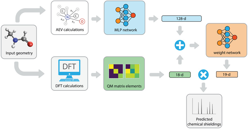
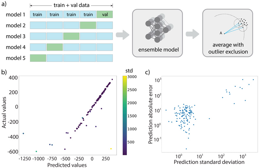
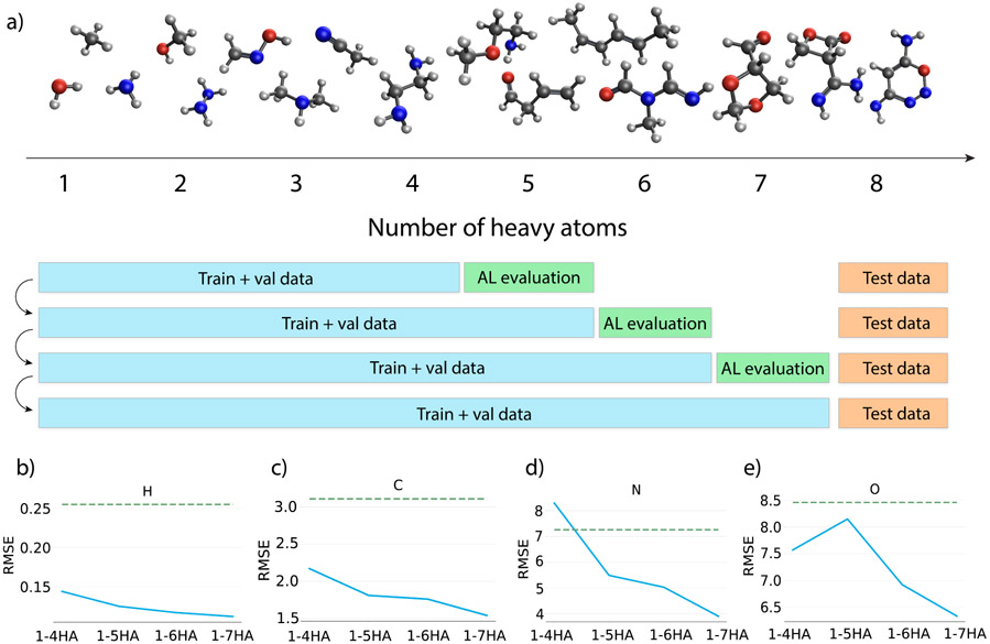
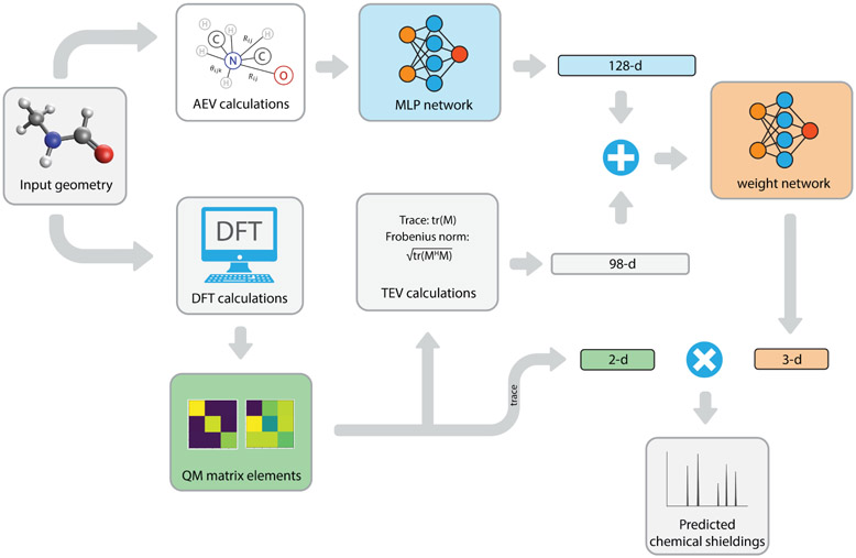
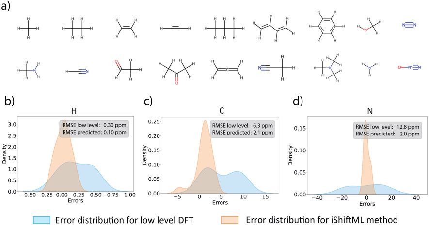
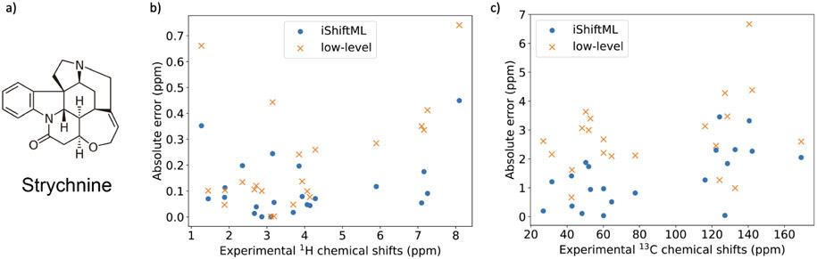
Theoretical predictions of NMR chemical shifts from first-principles can greatly facilitate experimental interpretation and structure identification of molecules in gas, solution, and solid-state phases. However, accurate prediction of chemical shifts using the gold-standard coupled cluster with singles, doubles, and perturbative triple excitations [CCSD(T)] method with a complete basis set (CBS) can be prohibitively expensive. By contrast, machine learning (ML) methods offer inexpensive alternatives for chemical shift predictions but are hampered by generalization to molecules outside the original training set. Here, we propose several new ideas in ML of the chemical shift prediction for H, C, N, and O that first introduce a novel feature representation, based on the atomic chemical shielding tensors within a molecular environment using an inexpensive quantum mechanics (QM) method, and train it to predict NMR chemical shieldings of a high-level composite theory that approaches the accuracy of CCSD(T)/CBS. In addition, we train the ML model through a new progressive active learning workflow that reduces the total number of expensive high-level composite calculations required while allowing the model to continuously improve on unseen data. Furthermore, the algorithm provides an error estimation, signaling potential unreliability in predictions if the error is large. Finally, we introduce a novel approach to keep the rotational invariance of the features using tensor environment vectors (TEVs) that yields a ML model with the highest accuracy compared to a similar model using data augmentation. We illustrate the predictive capacity of the resulting inexpensive shift machine learning (iShiftML) models across several benchmarks, including unseen molecules in the NS372 data set, gas-phase experimental chemical shifts for small organic molecules, and much larger and more complex natural products in which we can accurately differentiate between subtle diastereomers based on chemical shift assignments.

Figure 1:. The iShiftML ensemble learning model that uses low-level QM calculations of the shielding tensor and AEVs to predict high-level chemical shieldings.

Given a molecular geometry, the AEV around each nucleus is prepared and sent into a MLP network with two layers, each of which contains 128 neurons, in which the ReLU activation function is used for the first layer to encode the AEVs into a 128-dimension internal representation. On the second branch, we perform low-level composite QM calculations to obtain the 18 DIA and PARA chemical shielding values that are concatenated with the AEVs from the first branch to provide input for the second MLP weight network. The weight MLP is composed of a first layer containing 64 neurons and uses ReLU activation, followed by a second layer of 19 neurons (including a bias term) without an activation function.

Figure 2:. Distributions of weights of the original model without considering rotational invariance for hydrogen atom evaluated on test data.

Distributions of the weights for diagonal elements in the DIA and PARA matrices are centered close to 1/3, off-diagonal elements are centered around 0, and the bias term is distributed around −0.17.

Figure 3:. Ensemble prediction and correlation with actual prediction error.

(a) An ensemble learning approach using 5-fold cross-validation to train individual models in the ensemble. The final prediction is the average prediction from the models after excluding outliers recognized by the Local Outlier Factor algorithm. (b) An undertrained model for oxygen tested on the 8-heavy-atom test set, showing the correlation between predicted and actual values. Data points are colored according to their standard deviation (STD), with warm colors representing high STDs and cool colors representing low STDs. (c) Prediction errors compared to reference values are found to be well correlated with standard deviations of the predictions in the ensemble on a log-log plot. See Methods for further details.

Figure 4:. Procedure and results of the active learning workflow.

a) The active learning (AL) workflow. Starting from a model trained with data up to 4 heavy atoms (HA), data with 5HA are evaluated using the trained model, and 1500 structures with the largest predicted standard deviations from the 5HA dataset were included to define the training set for the next iteration until the training set contains molecules up to 7HA. The 8HA dataset was always used as the test set. b-e) RMSE on the 8HA test set for models trained with AL on training sets containing molecules with different sizes (blue curve), and also a baseline model that is trained using linear regression (green dotted line). Figures are for hydrogens (b), carbons (c), nitrogens (d) and oxygens (e). (b-e) are also provided in tabular form in Supplementary Table S2. Note that the RMSEs are calculated with uncertain predictions excluded, which removes any prediction with an ensemble standard deviation larger than 0.5 ppm for H, 2.5 ppm for C, 5 ppm for N, or 10 ppm for O.

Figure 5:. Architecture of the TEV variant of the iShift ML model.

As an alternative to the model in Figure 1, in the second branch the DIA and PARA chemical shielding tensors are embedded into a 98-dimension TEV vector that is concatenated with the AEVs from the first branch to provide input for the second MLP weight network. The weight MLP is composed of a first layer containing 64 neurons and uses ReLU activation, followed by a second layer of 3 neurons (including a bias term) without an activation function. In total, the TEV of one atom comprises 98 elements, including 16 reference magnitude indices each for isotropic diamagnetic and paramagnetic values, 32 indices for the final isotropic value, and 16 direction elements each for the diamagnetic and paramagnetic tensors. This combination ensures both magnitude and direction while maintaining rotational invariance.

Figure 6:. Predicting experimental gas phase chemical shifts for small organic molecules.

(a) the small molecules under investigation. 3D geometries of these molecules are taken from NS372 and NIST database. (b-d) Distributions of errors between predicted and experimental gas phase NMR chemical shifts for low-level DFT calculations ($\omega$B97X-V/pcSseg-1, blue distributions) and iShiftML predictions for the high-level CCSD(T) composite method (orange distributions) for hydrogens (b), carbons (c), and nitrogens (d). Also see Figure S3 and Table S6.

Figure 7:. Results on predicting and comparing CS for strychnine.

a) Molecular structure of strychnine. b) Absolute prediction error for the low-level DFT method and iShiftML across the experimental CS range for hydrogens. c) Absolute prediction error for the low-level DFT method and iShiftML across the experimental CS range for carbons. All predicted CS are re-referenced to have the same mean values as experimental measurements.

Figure 8:. Predictive analysis and comparison of chemical shifts for the 8 diastereomers of vannusal B.

a) Molecular structures of the 8 diastereomers of vannusal B. Reproduced from reference [ 82] Copyright 2011 American Chemical Society. b) The prediction RMSE margins for various vannusal B isomers. The bottom position in each bar represents comparison with the true experimental CS, while the top indicates a comparison to vannusal B CS in its native form, 5-2. Predictions were made using iShiftML, low-level DFT, and M06/pcS-2 (the latter from Ref. 82). Large bars with a low bottom therefore indicate good discrimination between predicted CS for the true structure against potential misidentification with CS of the native structure. All predicted CS are re-referenced to have the same mean values as experimental measurements. Also see Figure S5.

References

-
- Jacobsen NE NMR data interpretation explained: understanding 1D and 2D NMR spectra of organic compounds and natural products; John Wiley & Sons, 2016.
- Hore PJ Nuclear magnetic resonance; Oxford University Press, USA, 2015.
- Derome AE Modern NMR techniques for chemistry research; Elsevier, 2013.
- Wüthrich K. Protein structure determination in solution by NMR spectroscopy. J. Biol. Chem 1990, 265, 22059–22062. - PubMed
Grants and funding
LinkOut - more resources
Full Text Sources