A single-cell time-lapse of mouse prenatal development from gastrula to birth

Abstract

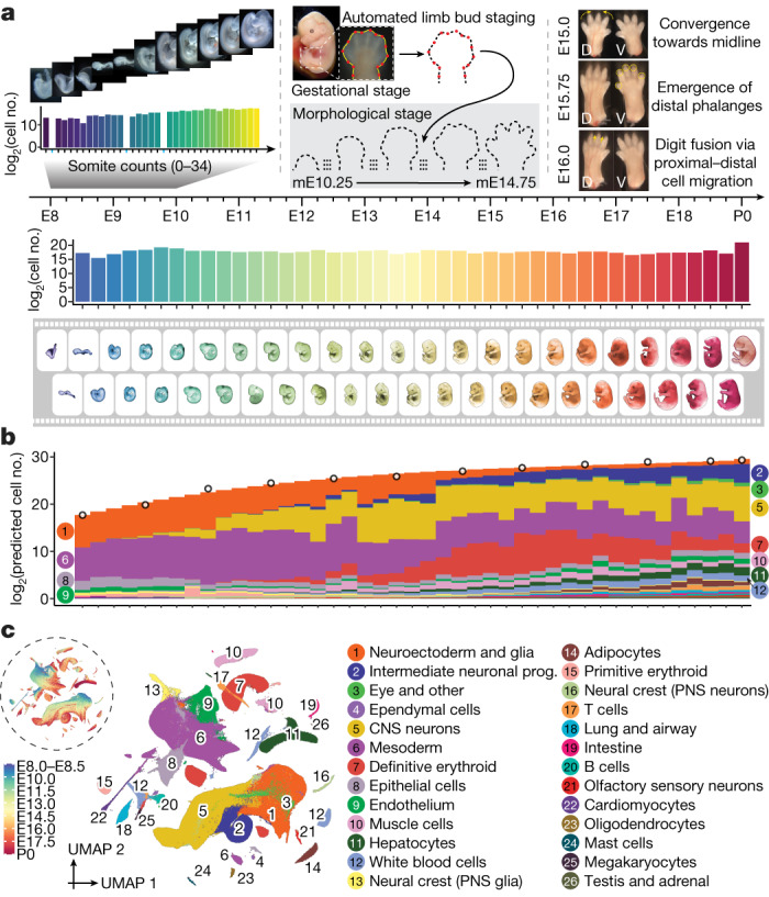
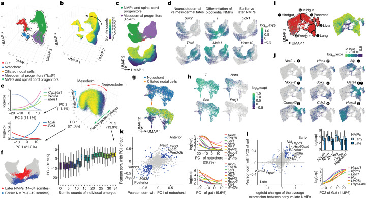
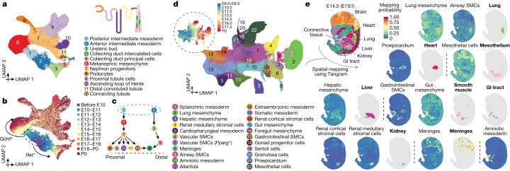
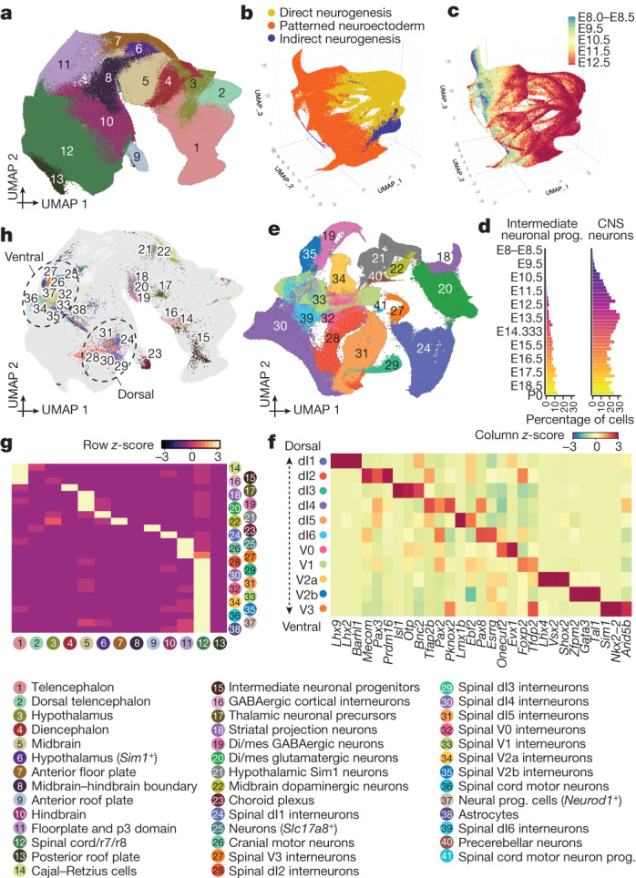
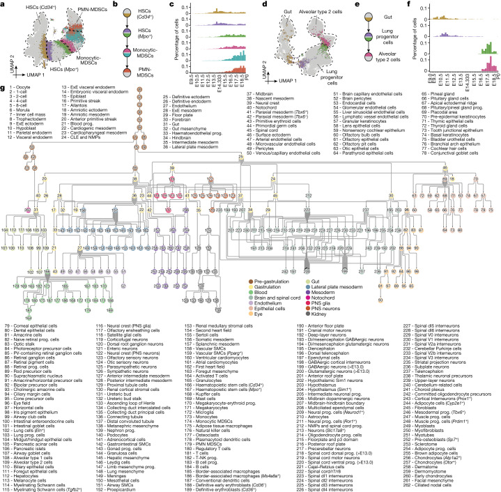
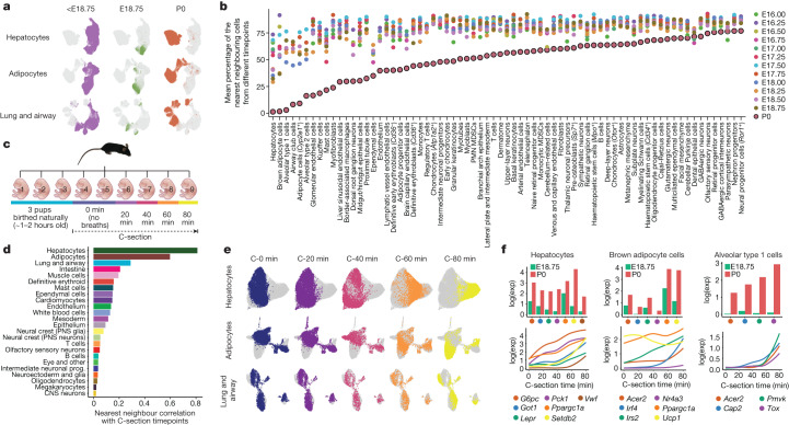
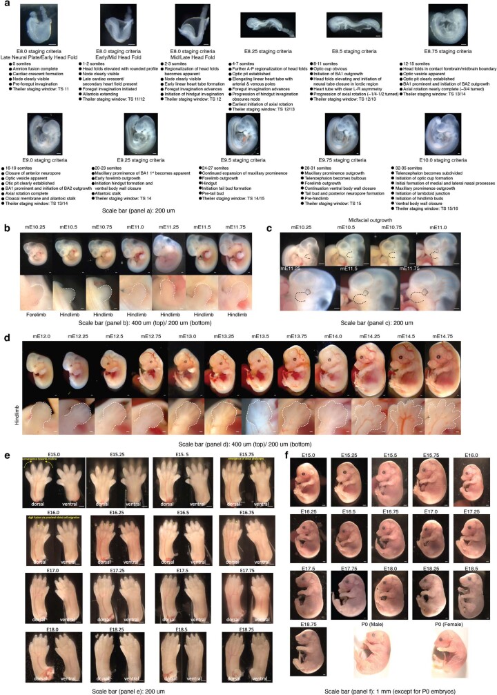
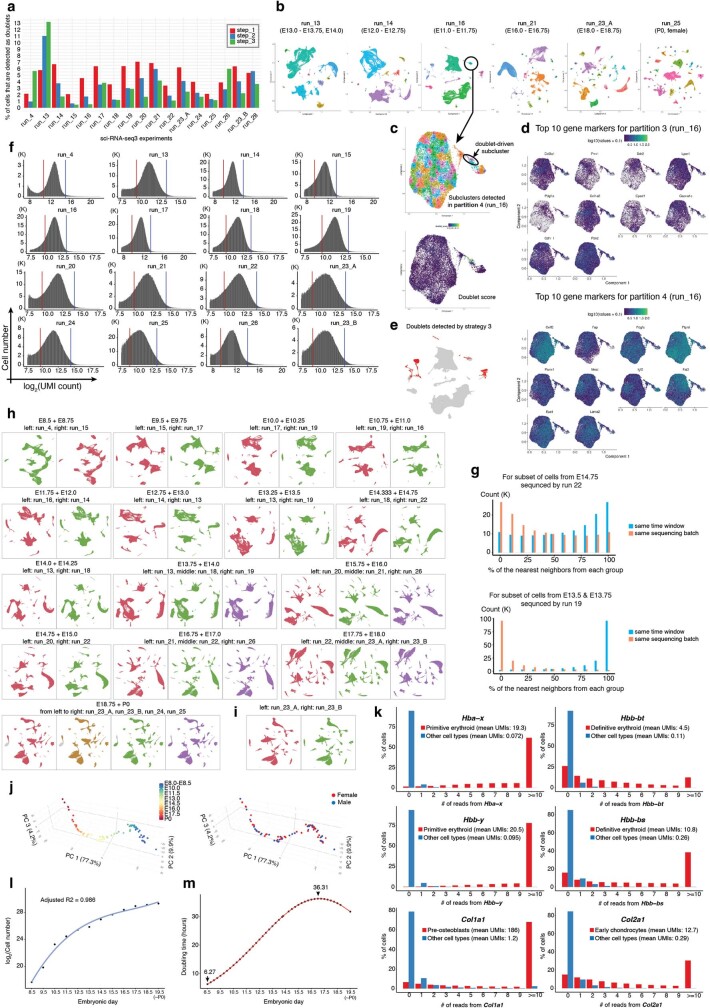
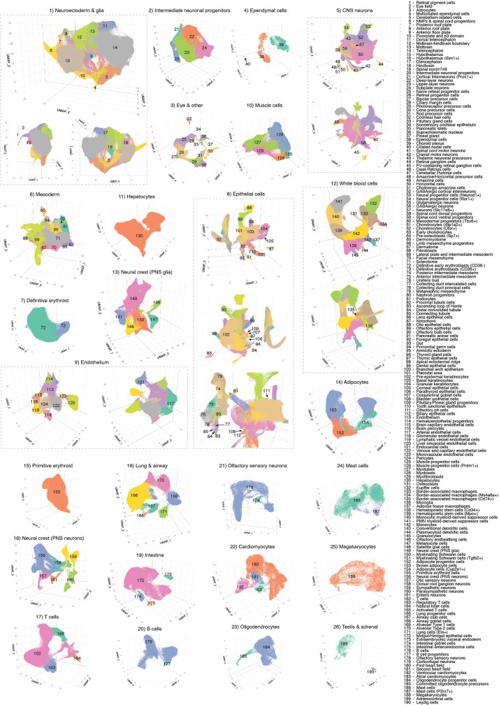
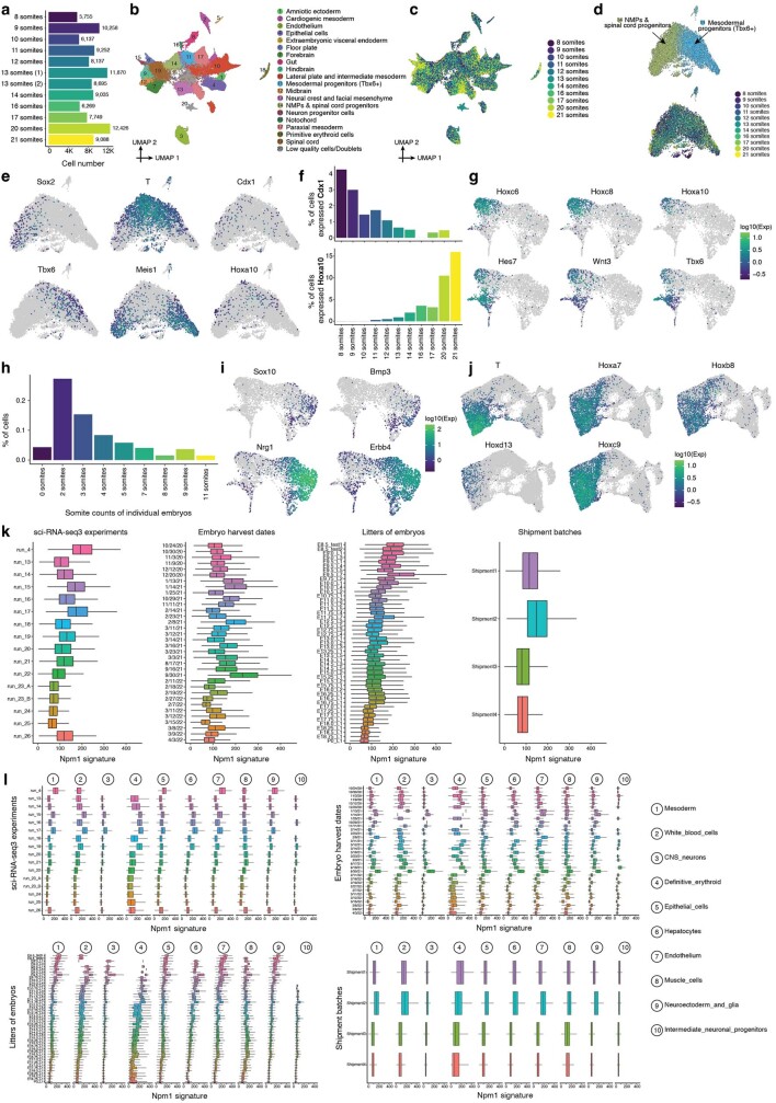
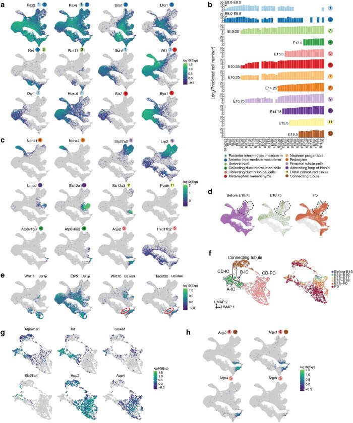
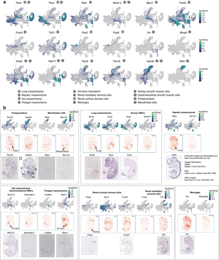
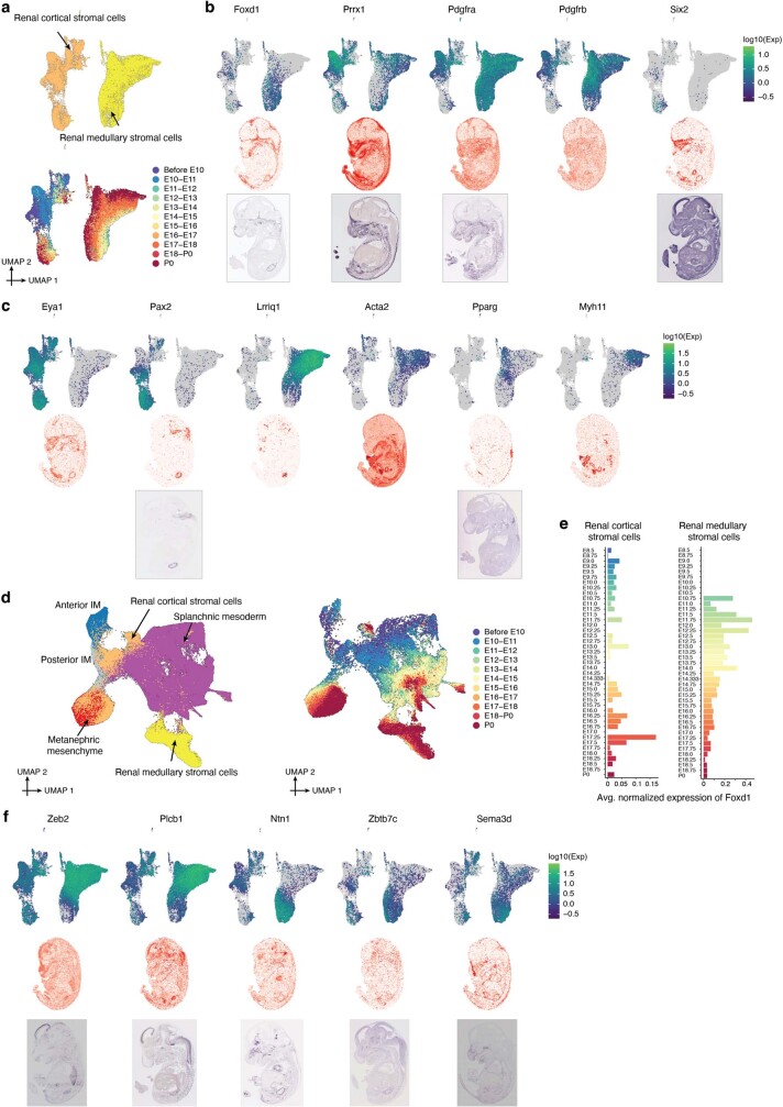
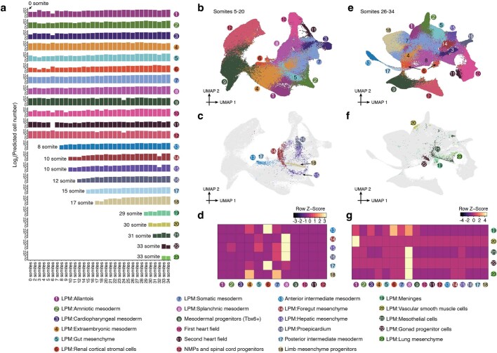
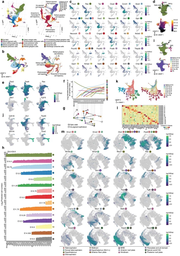
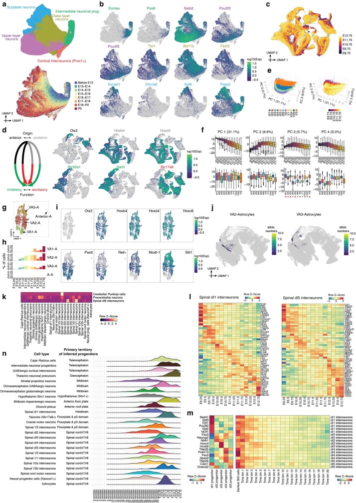
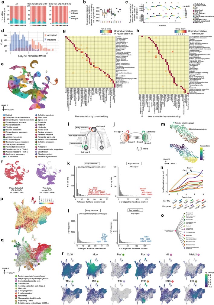
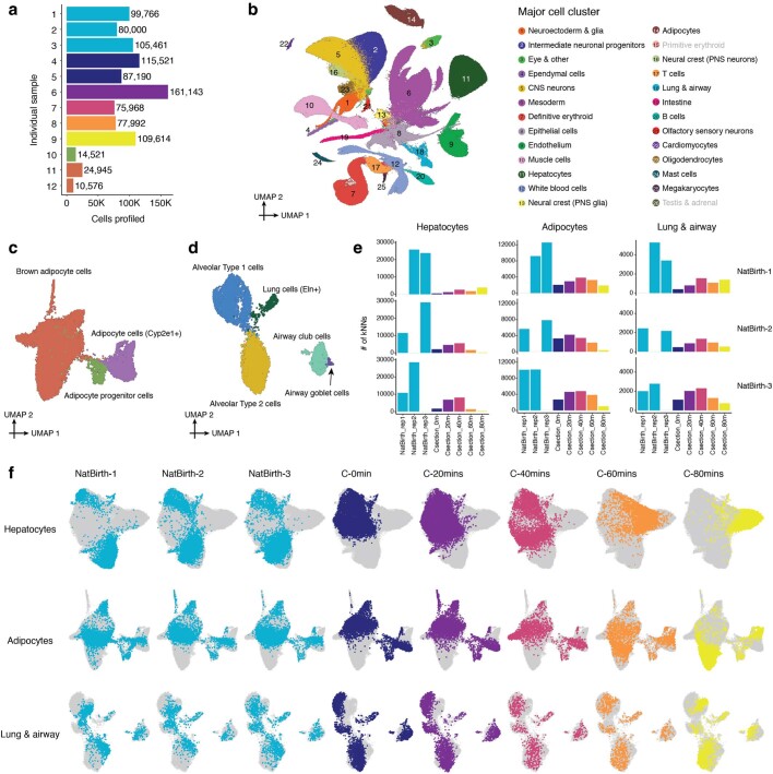
The house mouse (Mus musculus) is an exceptional model system, combining genetic tractability with close evolutionary affinity to humans^1,2. Mouse gestation lasts only 3 weeks, during which the genome orchestrates the astonishing transformation of a single-cell zygote into a free-living pup composed of more than 500 million cells. Here, to establish a global framework for exploring mammalian development, we applied optimized single-cell combinatorial indexing³ to profile the transcriptional states of 12.4 million nuclei from 83 embryos, precisely staged at 2- to 6-hour intervals spanning late gastrulation (embryonic day 8) to birth (postnatal day 0). From these data, we annotate hundreds of cell types and explore the ontogenesis of the posterior embryo during somitogenesis and of kidney, mesenchyme, retina and early neurons. We leverage the temporal resolution and sampling depth of these whole-embryo snapshots, together with published data^4-8 from earlier timepoints, to construct a rooted tree of cell-type relationships that spans the entirety of prenatal development, from zygote to birth. Throughout this tree, we systematically nominate genes encoding transcription factors and other proteins as candidate drivers of the in vivo differentiation of hundreds of cell types. Remarkably, the most marked temporal shifts in cell states are observed within one hour of birth and presumably underlie the massive physiological adaptations that must accompany the successful transition of a mammalian fetus to life outside the womb.

Fig. 1. A single-cell transcriptional time-lapse of mouse development, from gastrula to pup.

a, Embryos were collected and precisely staged based on morphological features, including by counting somite numbers (up to E10) and an automated process that leverages limb bud geometry (E10–E15) (Methods). Each embryo was assigned to one of 45 temporal bins at 6-h increments from E8 to P0, and to more highly resolved 2-h bins at earlier timepoints based on somite counts (0–34 somites). The first three bins (E8.0, E8.25 and E8.5) are combined. Embryos with somite counts 1, 13 and 19 are missing from the series (blue ticks in sub-axis). The number (log₂ scale) of nuclei profiled at each timepoint, is shown adjacent to the horizontal timeline, for 2-h bins (0–34 somites) for E8–E10 and for 6-h bins for E8–P0. b, Composition of embryos from each 6-h bin by major cell cluster. The y axis is scaled to the estimated cell number (log₂ scale) at each timepoint. In brief, we isolated and quantified total genomic DNA from whole embryos to estimate cell number at 12 stages (1-day bins, highlighted by black circles), and then predicted cell number at 43 timepoints using polynomial regression (Methods). c, Two-dimensional uniform manifold approximation and projection (UMAP) visualization of the whole dataset. The inset dashed circle shows the same UMAP coloured by developmental stage (plotting a uniform number of cells per timepoint). Colours and numbers in b,c correspond to the 26 listed major cell cluster annotations. Prog., progenitor. Source Data

Fig. 2. Transcriptional heterogeneity in the posterior embryo during early somitogenesis.

a, Re-embedded 3D UMAP of 121,118 cells from selected posterior embryonic cell types at early somitogenesis (somite counts 0–34; E8–E10). Three clusters are identified. b, The same UMAP as in a, coloured by somite counts. c, Re-embedded 2D UMAP of cells from cluster 1. d, The same UMAP as in c, coloured by marker gene expression for NMP subpopulations (Supplementary Table 12). Exp, expression. e, 3D visualization of the top three principal components of gene expression variation in cluster 1. Correlations between top three principal components and the normalized expression of selected genes (left) or somite counts (bottom). f, The same UMAP as in c, with earlier (n = 4,949 cells) and later (n = 3,910 cells) NMPs highlighted. NMPs: T⁺, (raw count ≥ 5) and Meis1⁻ (raw count = 0). g, Re-embedded 2D UMAP of cells from cluster 2. h, The same UMAP as in g, coloured by marker gene expression for notochord or ciliated nodal cells (Foxj1⁺). i, Re-embedded 2D UMAP of cells from cluster 3. Black circles highlight gut cell subpopulations. j, The same UMAP as in i, coloured by marker gene expression for gut cell subpopulations (Supplementary Table 12). k, Left, Pearson correlation (corr.) with PC1 of notochord or gut for highly variable genes. Right, gene expression of selected Wnt signalling genes versus PC1 of notochord or gut. l, Left, fold changes between early and late NMPs and Pearson correlation with PC2 of gut are plotted for highly variable genes. Right, gene expression of selected genes (several MYC targets, Lin28a and Hsp90aa1) versus early and late NMPs or PC2 of gut. In c,g,i, cells are coloured by either initial annotations or somite counts. Box plots in e (n = 98,545 cells) and l (n = 8,859 cells) represent inter-quartile range (IQR) (25th, 50th and 75th percentile) and whiskers represent 1.5× IQR. Source Data

Fig. 3. Diversification of the intermediate mesoderm and LPM.

a, Re-embedded 2D UMAP of 95,226 cells corresponding to renal development. A schematic of a nephron is shown at the top right. b, The same UMAP as in a, coloured by developmental stage (plotting a uniform number of cells per time window). The inset dashed circle highlights posterior and anterior intermediate mesoderm, with arrows highlighting derivative trajectories expressing Gdnf and Ret, respectively. c, Manually inferred relationships between annotated renal cell types. Label annotations in a. d, Re-embedded 2D UMAP of 745,494 cells from lateral plate and intermediate mesoderm derivatives. The inset dashed circle highlights the same UMAP with cells coloured by developmental stage. SMC, smooth muscle cell. e, The spatial origin of each lateral plate and intermediate mesoderm derivative was inferred based on a public dataset, Mosta, together with our data and the Tangram algorithm (Methods). An image of one selected section (E1S1) from E14.5 of the Mosta data is shown at the top left with major regions labelled. The spatial mapping probabilities across voxels on this section for selected subtypes are shown (non-bold label), with the regional annotation appearing to best correspond to the inferred spatial pattern shown alongside (labelled in bold). GI, gastrointestinal.

Fig. 4. The emergence of neuronal subtypes from the patterned neuroectoderm.

a, Re-embedded 2D UMAP of 1,185,052 cells, corresponding to different neuroectodermal territories from neuroectoderm and glia; major cell clusters, from stages before E13. b, Re-embedded 3D UMAP of 1,772,567 cells from neuroectodermal territories together with derived cell types, from stages before E13. Patterned neuroectoderm comprises neuroectoderm and glia and choroid plexus; direct neurogenesis comprises CNS neurons; indirect neurogenesis comprises intermediate neuronal progenitors. c, The same UMAP as in b, coloured by timepoint. d, Composition of embryos from each 6-h bin by intermediate neuronal progenitor (left) and CNS neuron (right) major cell clusters. e, Re-embedded 2D UMAP of 296,020 cells (glutamatergic neurons, GABAergic neurons, and spinal cord dorsal and ventral progenitors) from stages before E13. f, The top 3 transcription factor markers of the 11 spinal interneurons. Marker transcription factors were identified using the FindAllMarkers function of Seurat v3. The heat map shows mean gene expression values per cluster, calculated from normalized UMI counts. g, The row-scaled number of MNN pairs identified for each derivative cell type between its earliest 500 cells and cells from neuroectodermal territories. Some derivative cell types are excluded owing to low cell number or MNN pairs. h, The same UMAP as in a, but with inferred progenitor cells coloured by derivative cell type with the most frequent MNN pairs. Dotted circles highlight the dorsal and ventral spinal interneuron neurogenesis domains of the hindbrain and spinal cord. Di/mes, diencephalon and mesencephalon. Source Data

Fig. 5. A data-driven tree relating cell types throughout mouse development, from zygote to pup.

a, Illustration of the basis for the edge inference heuristic. Re-embedded 2D UMAP of 101,001 cells from Cd34⁺ HSCs, Mpo⁺ HSCs, monocytic myeloid-derived suppressor cells (MDSCs) and PMN MDSCs within the ‘blood’ subsystem. Cells involved in MNN pairs that bridge cell types are coloured. b, Inferred lineage relationships between annotated cell types in a, with corresponding colour scheme. c, The percentage of inter-cell-type MNN cells (y axis) versus the total number of cells profiled from embryos from the corresponding time bin, with colour scheme as in a,b. d, Additional illustration of the basis for the edge inference heuristic. Re-embedded 2D UMAP of 71,718 cells from gut, lung progenitor cells and alveolar type 2 cells within the ‘gut’ subsystem. Cells involved in MNN pairs that bridge cell types are coloured. e, Inferred lineage relationships between annotated cell types in d, with corresponding colour scheme. f, The percentage of inter-cell-type MNN cells (y axis) versus the total number of cells profiled from embryos from the corresponding time bin, with colour scheme as in d,e. g, A rooted, directed graph corresponding to development of a mouse, spanning E0 to P0 (Methods). For presentation purposes, we removed most ‘spatial continuity’ edges and merged nodes with redundant labels derived from different datasets, resulting in a rooted graph comprising 262 cell-type nodes and 338 edges. Nodes are coloured and labelled by each of the 14 subsystems. CLE, caudal lateral epiblast; ExE, extra-embryonic; NK-T cell, natural killer T cell; PV, parvalbumin. Source Data

Fig. 6. Rapid shifts in transcriptional state occur in a restricted subset of cell types upon birth.

a, Re-embedded 2D UMAP of cells from hepatocytes, adipocytes, and lung and airway, with colours highlighting cells from pre-E18.75 stages (left), E18.75 (middle) or P0 (right) embryos. b, We identified cell types with abrupt transcriptional changes before versus after birth by combining cells from animals collected after E16, performing PCA and calculating the average proportion of nearest neighbour cells from a different timepoint for each cell type (Methods). A low proportion of neighbours from different timepoints corresponds to a relatively abrupt change in transcriptional state. P0 points are highlighted with a black boundary. Differentially expressed genes for the 20 most highly ranked cell types are shown in Supplementary Table 25. c, A new scRNA-seq dataset (birth series) was generated from nuclei of pups collected after delivery (three vaginal births, six C-sections with 20-min increments). d, For each cell cluster in the birth series dataset, we calculated a Pearson correlation between the timepoint of each cell and the average timepoints of its ten nearest neighbours. High correlations indicate rapid, synchronized changes in transcriptional state. e, Re-embedded 2D UMAP of cells from hepatocytes, adipocytes, and lung and airway, based on cells from six pups delivered by C-section, with colours highlighting cells from pups collected after different intervals after delivery. f, Average normalized gene expression of selected genes for E18.75 versus P0 in the original data (top) and normalized expression of the same genes as a function of C-section timepoints (bottom) for hepatocytes, brown adipocyte cells and alveolar type 1 cells. Gene expression is normalized to total UMIs per cell and plotted as the natural logarithm. The line of gene expression was plotted using the geom_smooth function in ggplot2. Source Data

Extended Data Fig. 1. Embryos were collected and staged based on morphological features, including somite number and limb bud geometry.

a, Embryos harvested between E8 and E10 were precisely staged based upon somite counting. Harvested embryos were grouped into bins based on somite counting and further characterized based upon morphological features. Stage-representative images are shown with details of the main staging criteria for each coarse temporal bin listed. The approximately overlapping Theiler Stage (TS) is also noted for reference. Scale bar: 200 um. b, After E10, embryos were precisely staged based on morphological features. This was mainly done using the embryonic mouse ontogenetic staging system (eMOSS), an automated process that leverages limb bud geometry to infer developmental stage^,. Staging results derived from eMOSS are designated with “mE” for morphometric embryonic day. Specifically, for each temporal bin at 6-hr increments from E10.25-E11.75, an image of a stage-representative embryo is shown in the top row. Images of each embryo’s limb bud (white dashed outline) used for staging are shown in the bottom row. Scale bar: 400 um (top)/200 um (bottom). c, View of the craniofacial region of embryos shown in panel b demonstrates that limb bud staging also recreates the ordered ontogenetic progression of craniofacial morphogenesis, including development of the brain, eye, and outgrowth of facial prominences (black dashed line highlights maxillary process). Scale bar: 200 um. d, For each temporal bin at 6-hr increments from E12.0-E14.25, an image of a randomly selected embryo is shown in the top row. The subview of its hindlimb is shown in the bottom row. Scale bar: 400 um (top)/200 um (bottom). e, eMOSS is able to stage E10.25-E14.75, after which limb morphology becomes too complex. We defined additional dynamics related to digit formation to stage E15.0-E16.75 embryos. However, the remaining timepoints (E17.0-E18.75) were staged based upon gestational age. For each temporal bin at 6-hr increments from E15.0-E18.75, an image of the hindlimbs of a randomly selected embryo is shown. Scale bar: 200 um. f, For each temporal bin at 6-hr increments from E15.0-P0, an image of a stage-representative embryo is shown. Scale bar: 1 mm (except for P0 embryos).

Extended Data Fig. 2. Quality control on sci-RNA-seq3 experiments.

a, We performed three steps to detect and remove potential doublets from each single sci-RNA-seq3 experiment. First, we used Scrublet to calculate a doublet score for each cell. Cells with a doublet score over 0.2 were annotated as detected doublets. Second, we clustered and subclustered the entire dataset. Subclusters with a detected doublet ratio over 15% were annotated as doublet-derived subclusters. Third, after removing doublets detected by the first two steps, we performed clustering again to identify the major cell partitions (i.e. disjoint trajectories). Three experiments (runs 4, 15, and 17) that profiled embryos before E10 used cell clusters instead of cell partitions. We then generated a union gene list by combining the top 10 differentially expressed genes from each cell partition. This gene list was used to perform subclustering on each cell partition. Subclusters that showed low expression of target cell partition-specific markers and enriched expression of non-target cell cluster-partition markers were identified as doublet-driven clusters. More details are provided in the Methods. The percentage of cells detected and removed as doublets by each of the three steps in individual sci-RNA-seq3 experiments is shown. b, The labeled cell partitions for each of six selected experiments are shown, after removing doublets from the first two steps. c, Example of detection of doublet-driven subclusters via step 3. Re-embedded 2D UMAP of cells from partition 4 of experiment run_16, with cells colored by subclusters. The same UMAP is shown below, with cells colored by doublet score calculated by Scublet. d, The same UMAP as in panel c, colored by the normalized gene expression of the top 10 differentially expressed genes in either partition 3 (top) or partition 4 (bottom). e, The same UMAP as experiment run_16 in panel b, highlighted by doublets detected in step 3 (red). f, Histograms of log₂(UMI count) per single nucleus for each of 15 sci-RNA-seq3 experiments. For the 14 newly performed experiments (run_13 to run_26), upper (blue line) and lower (red line) thresholds used for quality filtering correspond to the mean plus 2 standard deviations and mean minus 1 standard deviation of log2-scaled values, respectively, after excluding cells with >85% of reads mapping to exonic regions (except for the lower bound of 500, which was manually assigned for run_25), are shown with vertical lines. The data of run_4, which was reported previously, was subjected to the same thresholds used in the original study, i.e. the mean +/− 2 standard deviations of log2-scaled values (blue and red vertical lines, respectively), after excluding cells with >85% of reads mapping to exonic regions. Run_23_A & B were from the same sci-RNA-seq3 experiment, but with nuclei which were sequenced separately. g, Although most of the embryos from the same approximate stage (e.g. E14.0-E14.75) were included in the same sci-RNA-seq3 experiment (Supplementary Table 1), we profiled extra nuclei in some experiments for a handful of timepoints to ensure sufficient coverage. Here we sought to leverage those instances to check for potential batch effects across experiments. For this, on the embedding learned from all of the data, we asked whether these cells’ profiles are more similar to cells from the same experiment or, alternatively, cells from the same time window. Top: for a random subset of cells from E14.75 which were profiled in experiment run_22 (primarily E17.0-E17.75), we performed a k-nearest neighbors (kNN, k = 10) approach in the global 3D UMAP to find the nearest neighboring cells either from the same experiment (red) or the same time window (E14.0-E14.75) but different experiment (blue). The percentages of the nearest neighboring cells from the two groups for individual cells are presented in the histogram. Bottom: a similar analysis was performed for a random subset of cells from E13.5 & E13.75 which were profiled in experiment run_19 (primarily E10.5-E11). In both examples, we observe that nearest neighbors are overwhelmingly cells from a different experiment (but the same time window), rather than cells from the same experiment (but a different time window). h, Cells processed in different experiments are well-integrated without batch correction. To further check for potential batch effects, we generated co-embeddings of samples processed from adjacent timepoints in different experiments, without batch correction. i, We also generated a co-embedding of cells from run_23_A (red) and run_23_B (green), which derived from the same sci-RNA-seq3 experiment but were sequenced on different NovaSeq runs. j, Embeddings of pseudo-bulk RNA-seq profiles of 74 mouse embryos in PCA space with visualization of top three PCs. Embryos are colored by either developmental stage (left) or data-inferred sex (right). k, Ambient noise (e.g. as might be due to transcript leakage) was assessed by examining hemoglobin and collagen transcripts. The distribution of the number of reads mapping to each selected hemoglobin or collagen gene across cells, for the cell type that is expected to express that gene at high levels (red) vs. all other cell types (blue). The mean UMI counts of cells in each group are also reported. The overall levels of ambient noise as assessed by these transcripts was low, e.g. the mean number of UMIs for Hbb-bs was 10.8 in definitive erythroid cells and 0.26 in all other cells, and for Col1a1 was 186 in pre-osteoblasts vs. 1.23 in all other cells. l, Quantitatively estimating cell number for individual mouse embryos as a function of developmental stage. Based on the experimentally estimated cell numbers of the 12 embryos (ranging from E8.5 to P0), we applied polynomial regression (degree = 3) to fix a curve across embryos between the embryonic day and log2-scaled cell number. P0 was treated as E19.5 in the model. m, The estimated “doubling time” of the total cell number in a whole mouse embryo are plotted as a function of timepoints. The timepoints with the longest (E17.0) and shortest (E8.5) estimated “doubling times” are highlighted. Source Data

Extended Data Fig. 3. Cell type annotations.

For each of the 26 major cell clusters, we performed subclustering and then annotated each of 190 subclusters using at least two literature-nominated marker genes per cell type label (Supplementary Table 5).

Extended Data Fig. 4. Transcriptional heterogeneity in the posterior embryo during early somitogenesis.

a, A validation sci-RNA-seq3 dataset of mouse embryos from somites 8 to 21. To validate findings related to differences between embryos staged with early vs. late somite counts, particularly in NMPs, we profiled another 12 precisely staged mouse embryos, ranging from 8 to 21 somites, in an independent sci-RNA-seq3 experiment. The resulting library was sequenced on an Illumina NextSeq 2000, resulting in 104,671 cells in total, with a median UMI count of 513 and a median gene count of 446 per cell. The number of cells profiled from each embryo. b, 2D UMAP visualization of the validation dataset (all cell types). c, The same UMAP as in panel b, with cells colored by somite count of the originating embryo. d, Re-embedded 2D UMAP of 9,686 cells from NMPs & spinal cord progenitors (cluster 11) and mesodermal progenitors (Tbx6 + ) (cluster 14) in panel b. Cells are colored by either the original annotation (top) or somite count (bottom). e, The same UMAP as in panel d, colored by gene expression of marker genes which appear specific to different subpopulations of NMPs: column 1: differences between neuroectodermal (Sox2 + ) vs. mesodermal (Tbx6 + ) fates; column 2: the differentiation of bipotential NMPs (T +, Meis1-) towards either fate; column 3: earlier (Cdx1 + ) vs. later (Hoxa10 + ) NMPs. References for marker genes are provided in Supplementary Table 12. f, Within the cells shown in panel d, the proportion of cells (y-axis) which express either Cdx1 (top) or Hoxa10 (bottom) are plotted as a function of somite count of the originating embryo. g, Transcriptional heterogeneity in the posterior embryo during the early somitogenesis. The same UMAP as in Fig. 2g, colored by gene expression of marker genes which appear specific to the subpopulation of notochord cluster that is Noto +, including posterior Hox genes (Hoxc6, Hoxc8, Hoxa10), and genes involved in Notch signaling (Hes7), Wnt signaling (Wnt3) and mesodermal differentiation (Tbx6). h, Cell proportions falling into the ciliated nodal cell cluster for embryos with different somite counts. i, The same UMAP as in Fig. 2g, colored by gene expression of marker genes which appear specific to the subpopulation of the notochord Noto- and more strongly Shh +, including Sox10, Bmp3, Nrg1, and Erbb4. j, The same UMAP as in Fig. 2i, colored by gene expression of marker genes which appear specific to the posterior gut endoderm, including T, Hoxa7, Hoxb8, Hoxd13, and Hoxc9. k, Checking the consistency of Npm1 signatures across different batches. First, we downsampled the dataset to ~1 M cells using geosketch and performed k-means clustering to ensure that each cluster contained roughly 500 cells. Second, we aggregated UMI counts for cells within each cluster to generate 2,289 meta-cells, and normalized the UMI counts for each meta-cell followed by log2-transformation. Third, we performed Pearson correlation between each protein-coding gene and Npm1, and selected genes with correlation coefficients > 0.6 (738 genes, ~3% of the total protein coding genes). A gene set enrichment analysis suggests that the module is associated with RNP complexes (corrected p-value = 1.4e-105), cytoplasmic translation (corrected p-value = 2.8e-90), and ribosomal proteins (corrected p-value = 7.4e-71). Finally, we summed the normalized UMI counts of these genes to calculate a Npm1 signature for individual cells. The resulting Npm1 signatures are subsetted in four plots, from left to right: by sci-RNA-seq3 experiment, embryo harvest date, litter of embryos, or shipment batch. l, Same as panel k, but further stratified by the top 10 abundant major cell clusters. Boxplots, in panel k (n = 1,144,141 cells) and l (n = 299,725 cells in Mesoderm, n = 127,150 cells in White blood cells, n = 104,205 cells in CNS neurons, n = 73,005 cells in Definitive erythroid, n = 66,772 cells in Epithelial cells, n = 64,845 cells in Hepatocytes, n = 62,951 cells in Endothelium, n = 61,249 cells in Muscle cells, n = 52,748 cells in Neuroectoderm and glia, n = 45,940 cells in Intermediate neuronal progenitors), represent IQR (25th, 50th, 75th percentile) with whiskers representing 1.5× IQR. Source Data

Extended Data Fig. 5. Transcriptional heterogeneity in renal development.

a, The same UMAP as in Fig. 3a, colored by expression of marker genes which appear specific to anterior intermediate mesoderm (Pax2 +, Pax8 +, Sim1 +, Lhx1 +, Ret +), posterior intermediate mesoderm (Pax2 +, Pax8 +, Gdnf1 +, Wt1 +, Osr1 +, Hoxc6 +), ureteric bud (Ret +, Wnt11 +) or metanephric mesenchyme (Wt1 +, Six2 +, Eya1 +). References for marker genes are provided in Supplementary Table 5. b, The predicted absolute number (log2 scale) of cells of each renal cell type at each timepoint. The predicted absolute number was calculated by the product of its sampling fraction in the overall embryo and the predicted total number of cells in the whole embryo at the corresponding timepoint (Fig. 1b). For each row, the first timepoint with at least 10 cells assigned that cell type annotation is labeled, and all observations prior to that timepoint are discarded. c, The same UMAP as in Fig. 3a, colored by expression of marker genes which appear specific to podocytes (Nphs1 +, Nphs2 +), proximal tubule cells (Slc27a2 +, Lrp2 +), ascending loop of Henle (Umod +, Slc12a1 +), distal convoluted tubule (Slc12a3 +, Pvalb +), collecting duct intercalated cells (Atp6v1g3 +, Atp6v0d2 +) or collecting duct principal cells (Aqp2 +, Hsd11b2 +). References for marker genes are provided in Supplementary Table 5. d, The same UMAP as Fig. 3a is shown three times, with colors highlighting cells from before E18.75 (left), E18.75 (middle), or P0 (right). Dotted cycles highlight cells which appear to correspond to the proximal tubule. e, The same UMAP as in Fig. 3a, colored by expression of marker genes which appear specific to the ureteric bud tip (Wnt11 +, Ret +, Etv5 +) or stalk (Wnt7b +, Tacstd2 +). Ureteric bud tip and stalk are highlighted by blue and red circles, respectively. f, Re-embedded 2D UMAP of 2,894 cells from connecting tubule cells, collecting duct principal cells (CD-PC), and collecting duct intercalated cells (CD-IC). Cells are colored by either their initial annotations (top) or timepoint (bottom). Black circles highlight the cells which appear to be either type A (A-IC) or type B (B-IC) intercalated cells. g, The same UMAP as in panel f, colored by expression of marker genes specific to CD-IC (Atp6v1b1 + ), A-IC (Kit +, Slc4a1 +), B-IC (Slc26a4 +), CD-PC (Aqp2 +, Aqp4 +), and connecting tubule (Aqp2 +, Aqp4-) (Supplementary Table 12). h, The same UMAP as in Fig. 3a, colored by expression of marker genes which appear specific to connecting tubule cells (Aqp2 +, Aqp3 +, Aqp4-) or collecting duct cells (Aqp2 +, Aqp3 +, Aqp4 +, Aqp5 +). Source Data

Extended Data Fig. 6. Transcriptional heterogeneity in mesenchyme.

a, The same UMAP as in Fig. 3d, colored by expression of marker genes which appear specific to lung mesenchyme (Tbx5 +, Tbx4 + ), hepatic mesenchyme (Reln + ), gut mesenchyme (Nkx2-3 + ), foregut mesenchyme (Barx1 + ), amniotic mesoderm (Postn + ), renal medullary stromal cells (Foxd1 +, Tcf21 + ), renal cortical stromal cells (Pax2 +, Pax8 + ), meninges (Vtn + ), airway smooth muscle cells (Trpc6 +, Tbx5 + ), gastrointestinal smooth muscle cells (Nkx2-3 + ), proepicardium or mesothelium (Msln + ). References for marker genes are provided in Supplementary Table 12. b, Published in situ hybridization (ISH) images support our annotations of lateral plate and intermediate mesoderm derivatives. In each subpanel (defined by dotted rectangles), three rows are shown for one or two lateral plate and intermediate mesoderm derivative cell types. Notably, each of these cell types was annotated based on spatial mapping analysis, as shown in Fig. 3e. Top: The same UMAP as in Fig. 3d, colored by gene expression of marker genes which appear specific to the given cell type. Middle: Virtual in situ hybridization (ISH) images of individual genes from one selected section (E1S1) from E14.5 of the Mosta data (https://db.cngb.org/stomics/mosta/). Bottom: In situ hybridization (ISH) images of individual genes were obtained from the Jackson Laboratory Mouse Genome Informatics (MGI) website (https://www.informatics.jax.org/). The original reference for these ISH images are^–.

Extended Data Fig. 7. Assessing the potential origins of LPM subsets annotated as renal cortical & medullary stromal cells.

a, Re-embedded 2D UMAP of 39,468 cells from renal cortical & medullary stromal cells. Cells are colored by either annotation (top) or timepoint (bottom, after downsampling to a uniform number of cells per time window). b, Top: The same UMAP as in panel a, colored by gene expression of marker genes which appear specific to renal cortical & medullary stromal cells. Both cell types express Foxd1, Prrx1, Pdgfra, and Pdgfrb, but only renal cortical stromal cells express Six2. Middle: Virtual in situ hybridization (ISH) images of individual genes. Bottom: ISH images of individual genes. c, Top: The same UMAP as in panel a, colored by gene expression of marker genes which appear specific to renal cortical stromal cells (Eya1 +, Pax2 + ), and renal medullary stromal cells (Lrriq1 +, Acta2 +, Pparg +, Myh11 + ). Middle: Virtual ISH images of individual genes. Bottom: ISH images of individual genes. d, Re-embedded 2D UMAP of 206,908 cells from renal cortical & medullary cells, anterior intermediate mesoderm, posterior intermediate mesoderm, metanephric mesenchyme, and splanchnic mesoderm. Cells are colored by either their initial annotations (left) or timepoint (right, after downsampling to a uniform number of cells per time window). e, The average normalized expression of Foxd1 over time is shown for renal cortical stromal cells (left) and renal medullary stromal cells (right). Gene expression was normalized by the size factor estimated by Monocle/3. f, Top: The same UMAP as in panel a, colored by gene expression of marker genes which appear specific to two subsets of renal stromal cells: medullary renal stromal cells (Zeb2 +, Plcb1 + ) and cortical renal stromal cells (Ntn1 +, Zbtb7c +, Sema3d + ), respectively. Middle: Virtual ISH images of individual genes. Bottom: ISH images of individual genes. In panel b, c, and f, virtual ISH images of individual genes were obtained from one selected section (E1S1) from E14.5 of the Mosta data (https://db.cngb.org/stomics/mosta/). ISH images were obtained from the Jackson Laboratory Mouse Genome Informatics (MGI) website (https://www.informatics.jax.org/). The original reference for these ISH images are^,,. Source Data

Extended Data Fig. 8. The emergence of mesenchymal subtypes from the patterned mesoderm.

a, The predicted absolute number (log2 scale) of cells of each mesoderm cell type at each somite count. The predicted absolute number was calculated by the product of its sampling fraction in the overall embryo and the predicted total number of cells in the whole embryo at the corresponding timepoint. Because cell numbers were only predicted for the broader bins (Fig. 1b), rather than individual somite counts, these were used for roughly corresponding sets (0-12 somite stage: E8.5; 14-15 somite stage: E8.75; 16-18 somite stage: E9.0; 20-23 somite stage: E9.25; 24-26 somite stage: E9.5; 27-31 somite stage: E9.75; 32-34 somite stage: E10.0). For each row, the first somite count with at least 10 cells assigned that cell type annotation is labeled, and all observations prior to that somite count are discarded. b, Re-embedded 2D UMAP of 110,753 cells from the selected cell types of mesoderm (clusters 1-12 as listed in panel a) from 5-20 somite stage embryos. c, The same UMAP as in panel b, but with inferred progenitor cells colored by derivative cell type with the highest mutual nearest neighbors (MNN) pairing score. d, Normalized MNN pairing score between mesodermal territories (column) and their inferred derivative cell types (row) from 5-20 somite stage embryos. The selected cell populations are first embedded into 30 dimensional PCA space, and then for individual derivative cell types, MNN pairs (k = 10 used for k-NN) between their earliest 500 cells (in absolute time) and cells from mesodermal territories are identified. e, Re-embedded 2D UMAP of 275,000 cells from the selected cell types of mesoderm (clusters 1-18 as listed in panel a) from 26-34 somite stage embryos. f, The same UMAP as in panel e, but with inferred progenitor cells colored by derivative cell type with the highest MNN pairing score. g, Normalized MNN pairing score between mesodermal territories (column) and their inferred derivative cell types (row) from 26-34 somite stage embryos. The selected cell populations are first embedded into 30 dimensional PCA space, and then for individual derivative cell types, MNN pairs (k = 10 used for k-NN) between their earliest 500 cells (in absolute time) and cells from mesodermal territories are identified. Source Data

Extended Data Fig. 9. The timing and trajectories of retinal development, and marker gene expression for different neuroectodermal territories.

a, Re-embedded 3D UMAP of 160,834 cells corresponding to the retinal development from E8 to P0. Cells are colored by either their initial annotations (left) or timepoint (right, after downsampling to a uniform number of cells per time window). Arrows highlight five of the main trajectories observed. b, Re-embedded 2D UMAP of 160,834 cells corresponding to the retinal development from E8 to P0. The same UMAP as in panel a, except 2D instead of 3D projection. c, The same UMAP as in panel b, colored by gene expression of marker genes for each annotated retinal cell type. References for marker genes are provided in Supplementary Table 5. d, Re-embedded 2D UMAP of the subset of cells in panel a from stages <= E12.5. Cells are colored by either their initial annotations (top) or timepoint (bottom). e, The same UMAP as in panel d, colored by gene expression of markers of retinal progenitor cells RPCs (Pax2 +, Pax6 +, Rax +, Fgf15 +), RPE (Tyr +), and the optic stalk (Pax2 +, Vax1 +, Rax−). References for marker genes are provided in Supplementary Table 12. f, Rescaled proportion of profiled cells (log2; y-axis) for each cell type shown in panel a, as a function of developmental time (x-axis). For rescaling, the % of profiled cells in the entire embryo assigned a given annotation was multiplied by 100,000, prior to taking the log2. Line plotted with geom_smooth function in ggplot2. g, Schematic of retinal cell types emphasizing the timing at which they first appear and their inferred developmental relationships from E8-P0, based on manual review of the trajectories. The gray lines indicate subsets of the eye field and RPE subsequently annotated as the optic stalk (label 16) and iris pigment epithelium (label 17), respectively. Cell types are positioned along the x-axis at the timepoint at which they are first observed (as shown in panel h). h, The predicted absolute number (log2 scale) of cells of each retinal cell type at each timepoint. The predicted absolute number was calculated by the product of its sampling fraction in the overall embryo and the predicted total number of cells in the whole embryo at the corresponding timepoint (Fig. 1b). For each row, the first timepoint with at least 10 cells assigned that cell type annotation is labeled, and all observations prior to that timepoint are discarded. i, Re-embedded 2D UMAP of a subset of cells in panel a corresponding to eye field, RPE and CMZ. Cells are colored by either their initial annotations (top) or timepoint (bottom). j, The same UMAP as in panel i, colored by gene expression of marker genes for IPE or pigment epithelium more generally (Tyr & Oca2). RPE: retinal pigment epithelium. CMZ: ciliary marginal zone. RPCs: retinal progenitor cells. IPE: iris pigment epithelium. References for marker genes are provided in Supplementary Table 12. k, Re-embedded 2D UMAP of retinal ganglion cells. Cells are colored by either clusters (left; Leiden clustering followed by downselection to late-appearing clusters) or timepoint (right). l, The top 3 TF markers of the 15 clusters shown in panel k. Marker TFs were identified using the FindAllMarkers function of Seurat/v3. Their mean gene expression values in each cluster are represented in the heatmap, calculated from original UMI counts normalized to total UMIs per cell, followed by natural-log transformation. The full list of significant TFs is provided in Supplementary Table 14. m, Marker gene expression for different neuroectodermal territories. The same UMAP as in Fig. 4a, colored by gene expression of marker genes for each neuroectodermal territory. References for marker genes are provided in Supplementary Table 5. Source Data

Extended Data Fig. 10. Subtypes of intermediate neuronal progenitors, glutamatergic & GABAergic neurons, and early astrocytes, and the timing of neuronal subtype differentiation from the patterned neuroectoderm.

a, Re-embedded 2D UMAP of 628,251 cells within the intermediate neuronal progenitors major cell cluster, colored by either cell type (top) or developmental stage (bottom, after downsampling to a uniform number of cells per time window). b, The same UMAP as in panel a, colored by gene expression of marker genes which appear specific to intermediate neuronal progenitors (Eomes +, Pax6 + ), upper-layer neurons (Satb2 +, Pou3f2 +, Pou3f3 + ), deep-layer neurons (Tbr1 +, Bcl11b +, Fezf2 + ), or subplate neurons (Kcnab1 +, Chrna5 +, Syt6 +, Foxp2 + ). References for marker genes are provided in Supplementary Table 5. c, The same UMAP as in Fig. 4e, with cells colored by timepoints. d, Left: Neuronal subtypes shown in Fig. 4e originate from anterior vs. posterior of neuroectoderm, and then subsequently display inhibitory vs. excitatory functions after differentiation. Right: The same UMAP as in Fig. 4e, colored by gene expression of marker genes which appear specific to anterior (Otx2 + ) vs. posterior (Hoxb4 +, Hoxd4 + ) origins, or inhibitory (Slc32a1 +, Gad1 + ) vs. excitatory (Slc17a6 + ) functions. References for marker genes are provided in Supplementary Table 12. e, 3D visualization of gene expression variation in 11 spinal interneurons, colored by cell type (left) or timepoint (right). f, Correlations between top four PCs and timepoints (top row) or cell types (bottom row). Boxplots (n = 97,842 cells) represent IQR (25th, 50th, 75th percentile) with whiskers representing 1.5× IQR. Red triangles and green stars highlight glutamatergic and GABAergic spinal cord interneurons, respectively. g, Subtypes of early astrocytes and their inferred progenitors. Re-embedded 2D UMAP of 5,928 cells within the astrocytes from stages <E13. h, Composition of embryos from each 6-hr bin by different subpopulations of astrocytes. i, The same UMAP as in panel g, colored by gene expression of marker genes which appear specific to anterior (Otx2 + ) or posterior (Hoxb4 +, Hoxd4 +, Hoxc6 + ) astrocytes, VA1-astrocytes (Pax6 +, Reln + ), VA2-astrocytes (Pax6 +, Reln +, Nkx6-1 +, Slit1 + ), and VA3-astrocytes (Nkx6-1 +, Slit1 + ). References for marker genes are provided in Supplementary Table 12. j, The same UMAP of the patterned neuroectoderm as in Fig. 4a, with inferred progenitor cells of astrocytes colored by the frequency that has been identified as a MNN with either VA2-astrocytes (left) or VA3-astrocytes (right). k, For those three cell types (cerebellar Purkinje cells, precerebellar neurons, spinal dI6 interneurons) which were excluded from the analyses represented in Fig. 4g, h due to having fewer than 50 MNN pairs, we performed a recursive mapping to identify whether they might share progenitors with another derived cell type, essentially repeating the analysis but attempting to map the earliest cells of these cell types to other derivative cell types rather than the patterned neuroectoderm. The heatmap shows the number of MNN pairs between pairwise cell types. In brief, this analysis suggests that spinal dl2 interneurons and cerebellar astrocytes share progenitors, while the progenitors of the other two re-analyzed cell types remain ambiguous. l, Gene expression across timepoints, for the specific TF markers of spinal dI1 (left) or spinal dI5 (right) interneurons. m, Left: gene expression for 18 selected TFs, across progenitor cells of dI1-5 from the neuroectodermal territories. Right: gene expression for 18 selected TFs across 21 time bins for dl1-5 spinal interneurons in which the TF has been nominated as marker TF. For individual spinal interneurons (each row), the first time bin involves the earliest 500 cells, then the left cells break into 20 bins ordered by their timepoints and with the same number of cells in each bin. Only cells from stages <E13 are included. n, For each neuronal subtype in Fig. 4g, h, we selected the annotation in the patterned neuroectoderm to which the most inferred progenitors had been assigned, and plotted the distribution of timepoints for that subset of inferred progenitors. Source Data

Extended Data Fig. 11. Identifying equivalent cell type nodes across datasets, and systematically nominating TFs and other genes for cell type specification.

a, The MNN approach used for graph construction is robust to subsampling and choice of the k parameter. The percentage of MNNs between different cell types, from the same embryo (blue) or from different embryos (red), is shown for each developmental system during organogenesis & fetal development, for all cells (left), cells from E8.0 to E10.0 (middle), or cells from E13.0 to E13.75 (right). b, The Spearman correlation coefficients of the normalized number of MNNs between cell types, comparing random subsampling of 80% of the cells to the full set of cells. The subsampling was repeated 100 times. The number of MNNs between cell types were normalized by the total number of possible MNNs between them. Boxplot (n = 1,200 correlation coefficients) represents IQR (25th, 50th, 75th percentile) with whiskers representing 1.5× IQR. Outliers are shown as the dots outside the whiskers. c, The Spearman correlation coefficients of the normalized number of MNNs between cell types, comparing various choices for k parameter (k = 5, 10, 20, 30, 40, 50) and the choice of k parameter (k = 15) when applying kNN to the developmental systems during organogenesis & fetal development. The number of MNNs between cell types were normalized by the total number of possible MNNs between them. Colors and numbers in panels a-c correspond to each developmental system annotations listed at the top right. d, 1,155 edges with the number of normalized MNNs > 1 were manually reviewed for biological plausibility. Histogram of edges that were accepted or rejected as a function of normalized MNN score. e, Integration of scRNA-seq profiles from gastrulation and early somitogenesis to identify equivalent cell type nodes across datasets generated by distinct technologies. 2D UMAP visualization of co-embedded cells, derived both from a gastrulation dataset based on cells from E6.5 to E8.5 generated on the 10x Genomics platform (n = 108,857 cells) and the earliest ~1% of this dataset (0-12 somite stage embryos) generated by sci-RNA-seq3 (n = 153,597 nuclei), after batch correction. This is essentially an updated version of an analysis that we have done previously. We performed clustering and cell type annotation on the integrated co-embedding, as shown. f, The same UMAP as in panel e is shown twice, with colors highlighting cells/nuclei from Pijuan-Sala’s dataset (left) or early somitogenesis (right). g, For cells from the original Pijuan-Sala’s dataset, we quantify and display the overlap between the original annotations and the new annotations shown in panel e. For each row, the proportions of cells that are distributed across each column are transformed to z-score. h, For nuclei from the early somitogenesis embryos, we quantify and display the overlap between the original annotations and the new annotations shown in panel e. These mappings were the basis for dataset equivalence edges between the “gastrulation” and 12 “organogenesis & fetal development” subsystems. For each row, the proportions of cells that are distributed across each column are transformed to z-score. CLE: Caudal lateral epiblast. NMPs: Neuromesodermal progenitors. i, A Waddington landscape cartoon illustrating how a cell type transition might be broken into three phases. j, Given a directional edge between two nodes, A → B, we identified the subset of cells within each node that were either MNNs of the other cell type (inter-node; groups 2 & 3) or MNNs of those cells (intra-node; groups 1 & 4). If A → B, this effectively models the transition as group 1 → 2 → 3 → 4. k, Histograms of the number of edges in which TFs are differentially expressed. The left histogram counts only genes when they are differentially expressed across the early phase of an developmental progression edge, while the right histogram counts genes when they are differentially expressed in any phase of all edges. l, Same as panel k, but for all genes rather than only TFs. m, Re-embedded 2D UMAP of 988 cells participating in groups 1-4 of the transition from anterior primitive streak → definitive endoderm. Cells are colored by either cell type annotations (top) or estimated pseudotime (bottom) using Monocle3. n, For cells in panel m, normalized gene expression of selected genes are plotted as a function of estimated pseudotime. Gene expression values were calculated from original UMI counts normalized to total UMIs per cell, followed by natural-log transformation. The line of gene expression was plotted by the geom_smooth function in ggplot2. We manually added an offset based on their expression at pseudotime = 0 to the y-axis for individual genes. o, A sub-graph of Fig. 5g, including hematopoietic stem cells (Cd34 + ) and 12 cell type nodes which appear derived from it. p, Re-embedded 2D UMAP of 37,750 cells from hematopoietic stem cells (Cd34 + ), colored by developmental stage (after downsampling to a uniform number of cells per stage). q, The same UMAP as in panel p, but with inferred progenitor cells (the cells participating in the MNNs that support the edges) colored by derivative cell type with the most frequent MNN pairs. r, The same UMAP as in panel p, colored by gene expression of selected top key TFs which were upregulated during the “early transition” for each derivative. Source Data

Extended Data Fig. 12. Rapid shifts in transcriptional state occur in a restricted subset of cell types upon birth, and differ between vaginally and C-section delivered pups.

a, The number of nuclei profiled for each animal shown in Fig. 6c. A small number of nuclei from additional fetal samples from the original set of experiments were also profiled for quality control (samples 10-12). b, 2D UMAP visualization of the birth-series dataset (n = 962,697 cells). Colors correspond to 26 major cell cluster annotations (Fig. 1b, c). Two major cell clusters (the primitive erythroid and testis & adrenal major cell clusters) shown in the original dataset but missed here are highlighted in gray. Primitive erythroid cells are not present at these timepoints and testis & adrenal cells are collapsed to the epithelial cells major cell cluster due to their low numbers. c, Re-embedded 2D UMAP of 19,696 cells of the adipocyte major cell cluster. d, Re-embedded 2D UMAP of 7,986 cells of the lung & airway major cell cluster. e, For these three major cell clusters, we co-embedded cells from three vaginally delivered pups (samples 1-3 in Fig. 6c) and six pups delivered by C-section (samples 4-9 in Fig. 6c), followed by subsetting a uniform number of cells per sample. For cells from each of the three vaginally delivered pups, we calculated the number of their 10 nearest neighbors in the PCA embedding (n = 30 dimensions) from other samples. f, Re-embedded 2D UMAP of cells from these three major cell clusters, based on cells from three vaginally delivered pups and six pups delivered by C-section. For each row, the same UMAP is shown multiple times, with colors highlighting cells from individual pups (or two pups, in the case of the 0-min C-section timepoint). Source Data

References

1. Silver, L. M. Mouse Genetics: Concepts and Applications (Oxford Univ. Press, 1995).
1. Mouse Genome Sequencing Consortium et al. Initial sequencing and comparative analysis of the mouse genome. Nature. 2002;420:520–562. doi: 10.1038/nature01262. - DOI - PubMed
1. Martin BK, et al. Optimized single-nucleus transcriptional profiling by combinatorial indexing. Nat. Protoc. 2023;18:188–207. doi: 10.1038/s41596-022-00752-0. - DOI - PMC - PubMed
1. Xue Z, et al. Genetic programs in human and mouse early embryos revealed by single-cell RNA sequencing. Nature. 2013;500:593–597. doi: 10.1038/nature12364. - DOI - PMC - PubMed
1. Mohammed H, et al. Single-cell landscape of transcriptional heterogeneity and cell fate decisions during mouse early gastrulation. Cell Rep. 2017;20:1215–1228. doi: 10.1016/j.celrep.2017.07.009. - DOI - PMC - PubMed