Using Instrumental Variables to Measure Causation over Time in Cross-Lagged Panel Models

Abstract

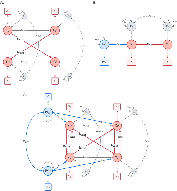
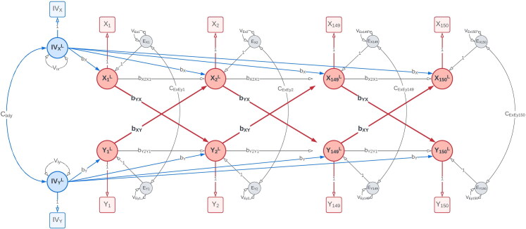
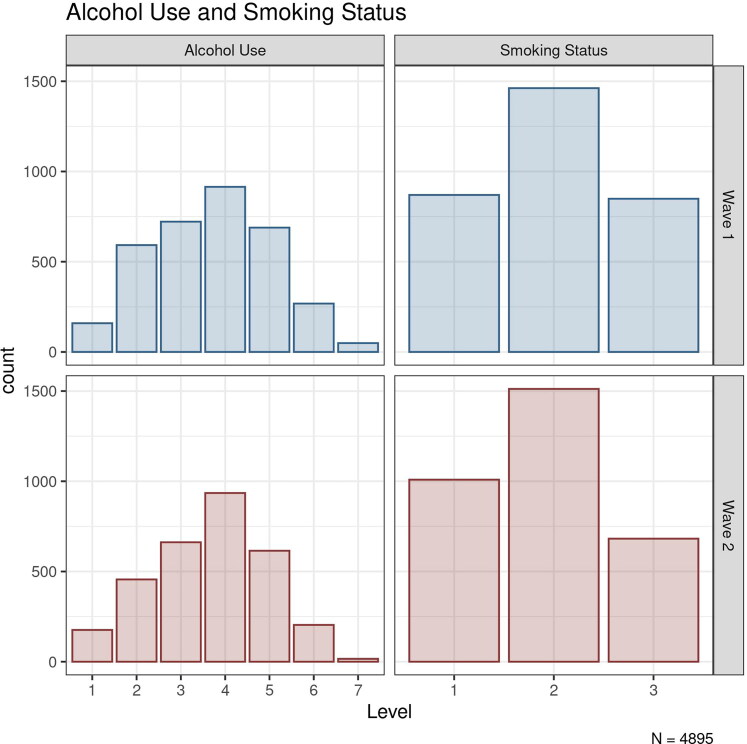
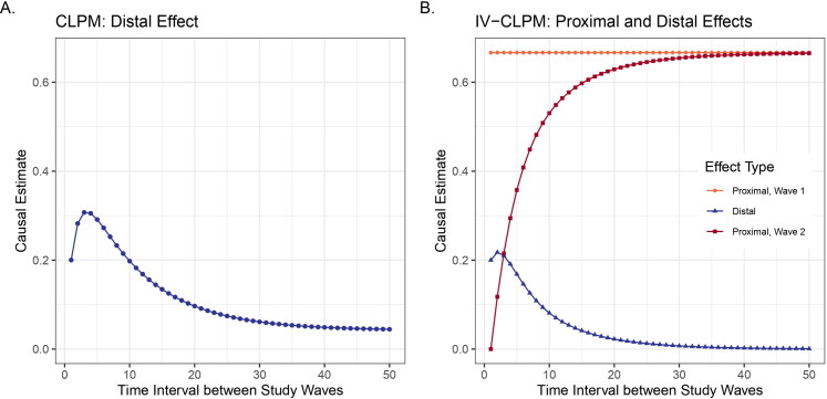
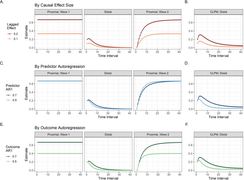
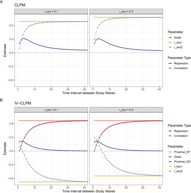
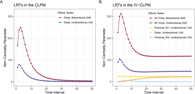
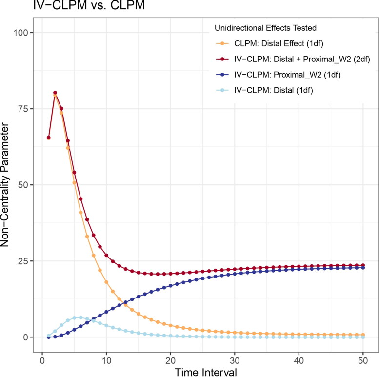
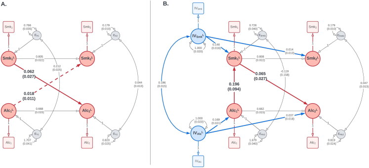
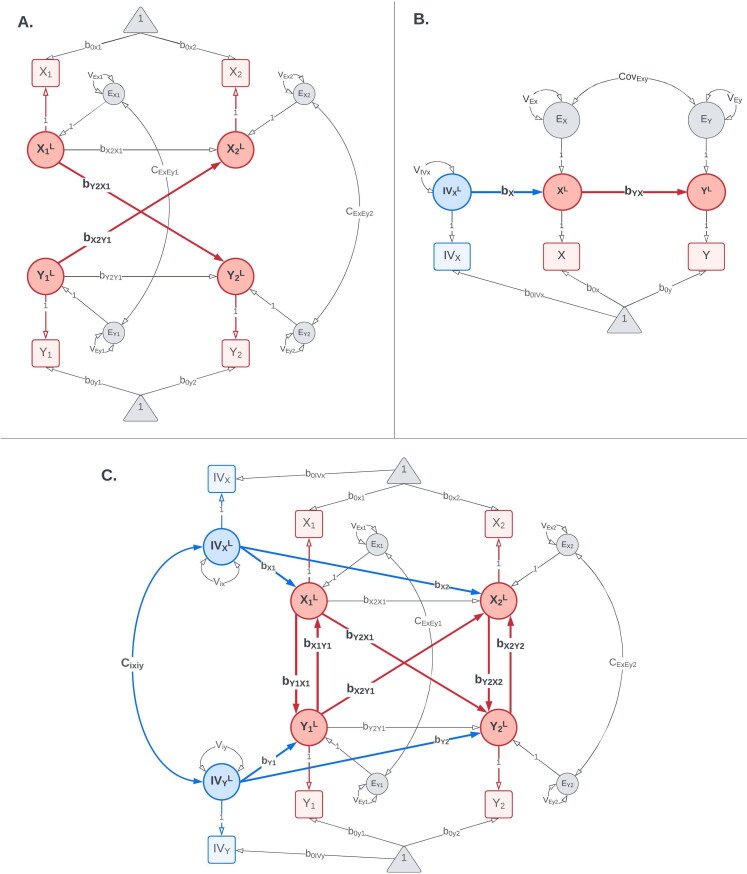
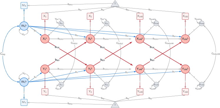
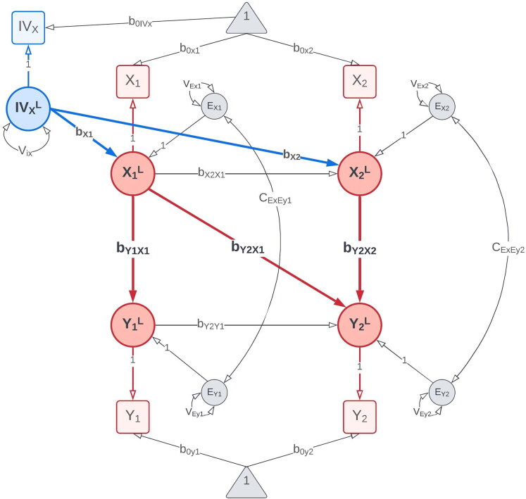
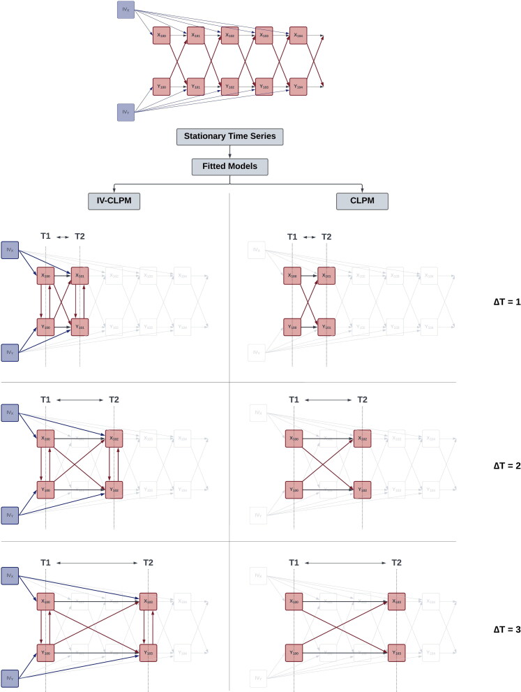
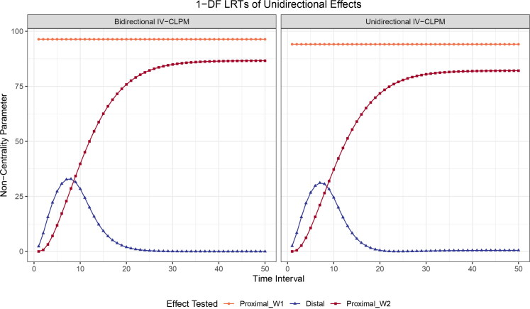
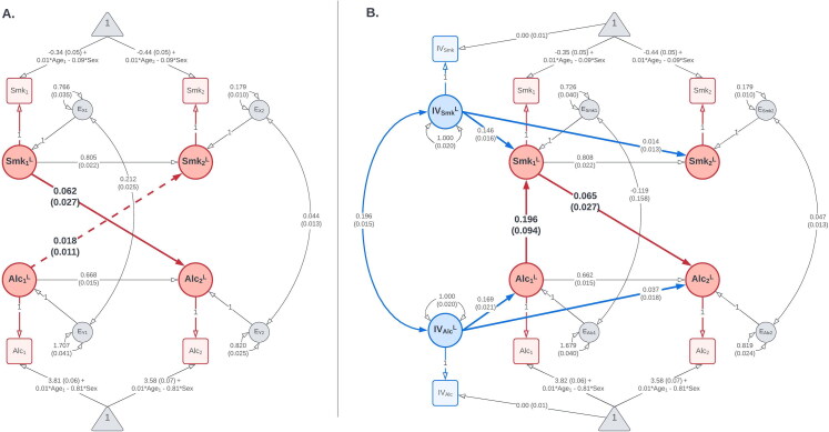
Cross-lagged panel models (CLPMs) are commonly used to estimate causal influences between two variables with repeated assessments. The lagged effects in a CLPM depend on the time interval between assessments, eventually becoming undetectable at longer intervals. To address this limitation, we incorporate instrumental variables (IVs) into the CLPM with two study waves and two variables. Doing so enables estimation of both the lagged (i.e., "distal") effects and the bidirectional cross-sectional (i.e., "proximal") effects at each wave. The distal effects reflect Granger-causal influences across time, which decay with increasing time intervals. The proximal effects capture causal influences that accrue over time and can help infer causality when the distal effects become undetectable at longer intervals. Significant proximal effects, with a negligible distal effect, would imply that the time interval is too long to estimate a lagged effect at that time interval using the standard CLPM. Through simulations and an empirical application, we demonstrate the impact of time intervals on causal inference in the CLPM and present modeling strategies to detect causal influences regardless of the time interval in a study. Furthermore, to motivate empirical applications of the proposed model, we highlight the utility and limitations of using genetic variables as IVs in large-scale panel studies.

Keywords: CLPM; Causal inference; instrumental variables; lagged effects.

Figure 1.

(A) CLPM: The cross-lagged panel model (CLPM) is used to estimate bidirectional lagged effects between X and Y ($b_{Y2X1}$ and $b_{X2Y1}$). This model was used as the reference model for integrating instrumental variables. (B) IV Regression: The instrumental variables regression (IVR) model fitted in a Structural Equation Modeling framework. The model uses the instrumental variable for X, IVx, to estimate the causal effect of X on Y ($b_{YX}$). (C) IV-CLPM: The proposed IV-CLPM model combines the CLPM with bidirectional IVR applied cross-sectionally at each wave. In addition to the lagged (i.e., “distal”) effects $b_{Y2X1}$ and $b_{X2Y1},$ the model utilizes IVR to estimate cross-sectional (i.e., “proximal”) effects at each wave: $b_{Y1X1}$ and $b_{X1Y1}$ at wave 1, and $b_{Y2X2}$ and $b_{X2Y2}$ at wave 2. In all three path diagrams, squares/rectangles represent the observed variables, and circles represent latent variables. To improve readability, the modeling of means is not shown in this figure. For complete path diagrams with means, please see Figure A1 in the Appendix A.

Figure 2.

Data-generating model: The data-generating model with bidirectional first-order causal effects between X and Y ($b_{YX}$ and $b_{XY}$) simulated over 150 time points. The instrumental variable for X, IVx, has an unchanging direct effect on X ($b_X$) at every time point. Likewise, the instrumental variable for Y, IVy, directly affects Y ($b_Y$) at all time points. Squares/rectangles represent the observed variables, and circles represent latent variables (i.e., the variances in this model). To improve readability, the modeling of means is not shown in this figure. For a complete path diagram with means, please see Figure A2 in the Appendix A.

Figure 3.

The univariate distributions of alcohol use and smoking status variables at wave 1 (Adult NTR survey 8) and wave 2 (Adult NTR survey 10) in the Netherlands Twin Register data used in our empirical example. Alcohol use was operationalized as the number of alcoholic drinks per week, with the seven levels corresponding to <1, 1–2, 3–5, 6–10, 11–20, 21–40, and >40 drinks per week, respectively. The cigarette smoking status variable was a categorical variable with three response options: 1 = “Never smoked regularly,” 2 = “Used to smoke but quit” (i.e., former smoking), and 3 = “Currently Smoking.”

Figure 4.

Impact of the time interval on (A) the distal effect in CLPM and (B) the distal and the two proximal effects in the IV-CLPM, with both models fitted to the data generated using the model in Figure 2. In the CLPM (A), the distal effect estimated increases briefly and then decreases asymptotically with increasing time intervals, varying from around 0.3 at an interval of 4 units to <0.05 at intervals longer than 30 units. In the IV-CLPM (B), the distal effect follows a pattern like that in the CLPM, but while the distal effect decays at longer intervals, the proximal effects can help estimate the causal effects. The plots illustrate the estimates for the effect of X on Y, given the first-order causal effect of X on Y = 0.2, the effect of Y on X = 0.2, first-order autoregression (AR1) of X = 0.7, AR1 of Y = 0.7, and the correlation between the residuals of X and Y = 0.3.

Figure 5.

The estimated causal effect of X on Y in the IV-CLPM (Figure 1(C)) and the CLPM (Figure 1(A)) at varying time intervals between study waves, given different levels of the first-order (i.e., at $\Delta T=1$) causal effect of X on Y (A,B), first-order autoregression (AR1) of predictor X (C,D), and AR1 of outcome Y (E,F) in the data-generating model (Figure 2). For ease of display, the time intervals are shown up to 40 units, by which point all parameter estimates are close to their asymptotes. (A,B) The first-order causal effect does not impact the rate at which the distal effect decays with increasing time intervals in either model. However, a larger first-order causal effect size does lead to larger causal estimates in both models (as expected). Note, though, that the distal effect in the IV-CLPM approaches zero at longer intervals, regardless of the first-order causal effect size. (C,D) A larger AR1 parameter (i.e., greater stability over time) of the predictor variable leads to a larger distal effect in the CLPM across time intervals, as well as slower decay of the distal effect with increasing intervals. On the contrary, the degree of AR1 in the predictor has minimal impact on the causal estimates in the IV-CLPM. Note that in panel C, the two curves for the Proximal Effect at Wave 1 have fully overlapped, so only one of the two curves is visible. (E,F) The AR1 parameter of the outcome variable impacts the causal estimates in both models: a higher level of outcome AR1 leads to larger causal estimates and slower decay of the distal effect in both models.

Figure 6.

Variation in the causal estimates (effect of X on Y) and the cross-sectional correlation between the residuals of X and Y in (A) the CLPM and (B) the IV-CLPM, at varying levels of correlation between the residuals in the data (r_exy). The residual correlation in the data has a negligible impact on the causal estimates in either model, but affects the correlation of the residuals in the model, r_exy1 and r_exy2. Given stationarity, the correlation of the residuals also varies with changes in the causal estimates, which, in turn, depend on the time interval between study waves. For ease of display, the time intervals are shown up to 40 units, by which point all parameter estimates are close to their asymptotes.

Figure 7.

Likelihood-ratio tests (LRTs) of the causal estimates in the traditional CLPM and the IV-CLPM at varying time intervals between study waves. (A) CLPM: The non-centrality parameter (NCP) obtained from a 2-degrees-of-freedom (2df) test of bidirectional distal effects, and that obtained from a 1df LRT of a unidirectional distal effect (shown here is X to Y). (B) IV-CLPM: The NCP from a 6df omnibus test of bidirectional causal estimates of three types: the proximal effect at wave 1 (Proximal_W1), the distal effect, and the proximal effect at wave 2 (Proximal_W2). A significant omnibus test is followed up with a 3df LRT of the three causal effects in each direction, and, finally, the 1df LRTs of the three causal effects separately (in each direction of causation). The NCPs were obtained by fixing to zero the parameters of interest in models fitted to data with $N=1000,$ $b_{YX}=0.2,$ $b_{XY}=0.$2, $b_{X2X1}=0.7,$ $b_{Y2Y1}=0.7,$ and $r_{\mathit{exy}}=0.3.$

Figure 8.

Comparison of the IV-CLPM’s joint test of (unidirectional) distal and wave-2 proximal effects with its 1df LRT of wave-2 proximal effect, as well as with the CLPM’s 1df LRT of distal effect. For reference, the IV-CLPM’s 1df LRT of distal effect is also shown. Comparing the 2df LRT statistic (dark red) with the 1df LRT of wave-2 proximal effect (dark blue) in the IV-CLPM can help gauge whether a particular time interval would be appropriate for fitting the traditional CLPM. The non-centrality parameters were obtained by fixing to zero the parameters of interest in models fitted to data with $N=1000,$ $b_{YX}=0.2,$ $b_{XY}=0.$2, $b_{X2X1}=0.7,$ $b_{Y2Y1}=0.7,$ and $r_{\mathit{exy}}=0.3.$

Figure 9.

Results of (A) the CLPM and (B) the best-fitting IV-CLPM examining bidirectional causal effects between smoking status (Smk) and alcoholic drinks per week (Alc), assessed three years apart. The paths have been labeled with the point estimate and its standard error (in parentheses). The dashed path in the CLPM indicates a non-significant causal estimate. The CLPM suggests a likely unidirectional causal process, with a significant effect of smoking on alcohol use, but not vice versa. On the contrary, the IV-CLPM suggests a more complex bidirectional causation, with a significant proximal effect of alcohol use on smoking, which, in turn, has a reciprocal distal effect on alcohol use. In both path diagrams, squares/rectangles represent the observed variables, and circles represent latent variables. To improve figure readability, means and covariates are not shown in this figure. For a complete path diagrams with means and covariates, please see Figure A6 in the Appendix A.

Figure A1.

(A) CLPM (with means): The cross-lagged panel model (CLPM) is used to estimate bidirectional lagged effects between X and Y ($b_{Y2X1}$ and $b_{X2Y1}$). This model was used as the reference model for integrating instrumental variables. (B) IV Regression (with means): The instrumental variables regression (IVR) model fitted in a Structural Equation Modeling framework. The model uses the instrumental variable for X, IVx, to estimate the causal effect of X on Y ($b_{YX}$). (C) IV-CLPM (with means): The proposed IV-CLPM model combines the CLPM with bidirectional IVR applied cross-sectionally at each wave. In addition to the lagged (i.e., “distal”) effects $b_{Y2X1}$ and $b_{X2Y1},$ the model utilizes IVR to estimate cross-sectional (i.e., “proximal”) effects at each wave: $b_{Y1X1}$ and $b_{X1Y1}$ at wave 1, and $b_{Y2X2}$ and $b_{X2Y2}$ at wave 2. In all three path diagrams, squares/rectangles represent the observed variables, and circles represent latent variables. Triangles represent constants used to model the variables’ mean levels.

Figure A2.

Data-generating model (with means): The data-generating model with bidirectional first-order causal effects between X and Y ($b_{YX}$ and $b_{XY}$) simulated over 150 time points. The instrumental variable for X, IVx, has an unchanging direct effect on X ($b_X$) at every time point. Likewise, the instrumental variable for Y, IVy, directly affects Y ($b_Y$) at all time points. Squares/rectangles represent the observed variables, and circles represent latent variables (i.e., the variances in this model). Triangles represent constants used to model the variables’ mean levels.

Figure A3.

Unidirectional IV-CLPM. The model combines a unidirectional version of the two-wave Cross-Lagged Panel Model (CLPM) with Instrumental Variables Regression (IVR) applied cross-sectionally at each wave. In addition to the lagged (i.e., “distal”) effect of X on Y ($b_{Y2X1}$), the model utilizes IVR to estimate cross-sectional (i.e., “proximal”) effects at each wave: $b_{Y1X1}$ at wave 1, and $b_{Y2X2}$ at wave 2. The squares/rectangles represent the observed variables, and circles represent latent variables. Triangles represent constants used to model the variables’ mean levels.

Figure A4.

Schematic of the study design for examining the impact of time interval on the causal inference in the proposed IV-CLPM and the traditional CLPM models. A stationary time series was generated with two constructs (X and Y) and their respective instrumental variable (IVx and IVy) with bidirectional first-order lagged effects between X and Y. To this data, a series of two-wave IV-CLPM and CLPM models were fitted. Across the models, the first wave (T1) was fixed at an arbitrary time-point in the stationary time series, while the second wave (T2) was changed by an increment of one unit in every successive model. In so doing, the time interval ($\Delta T=T2-T1$) in the fitted models was increased sequentially from 1 through 50. This figure depicts the models with $\Delta T=1,$ 2, and 3.

Figure A5.

Likelihood-ratio tests (LRTs) of the effects of X on Y in the bidirectional (left) and unidirectional (right) versions of the IV-CLPM, given data with unidirectional effects of X on Y. The non-centrality parameters were obtained by fixing to zero the causal parameters in models fitted to data with $N=1000,$ $b_{YX}=0.4,$ $b_{XY}=0,$ $b_{X2X1}=0.8,$ $b_{Y2Y1}=0.8,$ and $r_{\mathit{exy}}=0.3.$

Figure A6.

Results of (A) the CLPM (with means and covariates) and (B) the best-fitting IV-CLPM (with means and covariates) examining bidirectional causal effects between smoking status (Smk) and alcoholic drinks per week (Alc), assessed three years apart. The paths have been labeled with the point estimate and its standard error (in parentheses). The dashed path in the CLPM indicates a non-significant causal estimate. The CLPM suggests a likely unidirectional causal process, with a significant effect of smoking on alcohol use, but not vice versa. On the contrary, the IV-CLPM suggests a more complex bidirectional causation, with a significant proximal effect of alcohol use on smoking, which, in turn, has a reciprocal distal effect on alcohol use. In both path diagrams, squares/rectangles represent the observed variables, and circles represent latent variables. Triangles represent constants used to model the traits’ mean levels.

References

1. Akaike, H. (1974). A new look at the statistical model identification. IEEE Transactions on Automatic Control, 19(6), 716–723. 10.1109/TAC.1974.1100705 - DOI
1. Allison, P. D., Williams, R., & Moral-Benito, E. (2017). Maximum likelihood for cross-lagged panel models with fixed effects. Socius: Sociological Research for a Dynamic World, 3, 237802311771057. 10.1177/2378023117710578 - DOI
1. Amin, S., Korhonen, M., & Huikari, S. (2023). Unemployment and mental health: An instrumental variable analysis using municipal-level data for Finland for 2002–2019. Social Indicators Research, 166(3), 627–643. 10.1007/s11205-023-03081-1 - DOI
1. Andersen, H. K. (2022). Equivalent approaches to dealing with unobserved heterogeneity in cross-lagged panel models? Investigating the benefits and drawbacks of the latent curve model with structured residuals and the random intercept cross-lagged panel model. Psychological Methods, 27(5), 730–751. 10.1037/met0000285 - DOI - PubMed
1. Audrain-McGovern, J., Leventhal, A. M., & Strong, D. R. (2015). The role of depression in the uptake and maintenance of cigarette smoking. In De Biasi M. (Ed.), International review of neurobiology (Vol. 124, pp. 209–243). Academic Press. 10.1016/bs.irn.2015.07.004 - DOI - PMC - PubMed