The role of prospective contingency in the control of behavior and dopamine signals during associative learning

Abstract

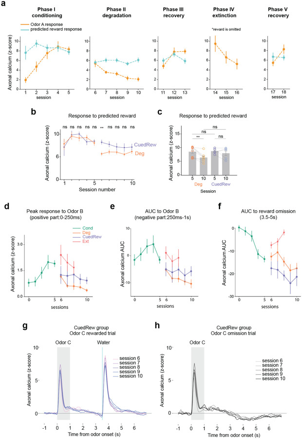
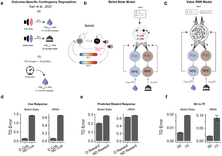
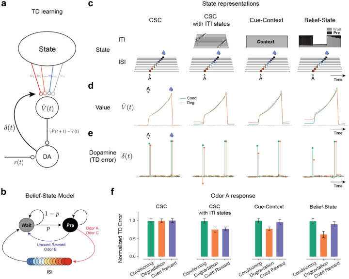
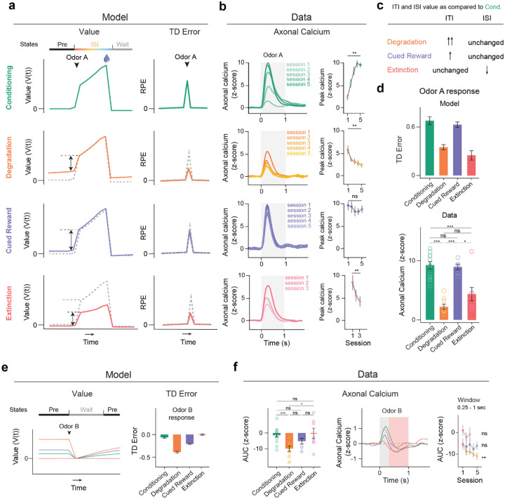
Associative learning depends on contingency, the degree to which a stimulus predicts an outcome. Despite its importance, the neural mechanisms linking contingency to behavior remain elusive. Here we examined the dopamine activity in the ventral striatum - a signal implicated in associative learning - in a Pavlovian contingency degradation task in mice. We show that both anticipatory licking and dopamine responses to a conditioned stimulus decreased when additional rewards were delivered uncued, but remained unchanged if additional rewards were cued. These results conflict with contingency-based accounts using a traditional definition of contingency or a novel causal learning model (ANCCR), but can be explained by temporal difference (TD) learning models equipped with an appropriate inter-trial-interval (ITI) state representation. Recurrent neural networks trained within a TD framework develop state representations like our best 'handcrafted' model. Our findings suggest that the TD error can be a measure that describes both contingency and dopaminergic activity.

Extended Data Fig. 1 |. Population Average Behavior per session

(a, b, c, d) Bar graphs comparing the average number of licks to Odor A during the first 3s post-stimulus (a) and during ITI (b), latency to lick (c), and fraction correct (d) in the final sessions of phase 1 and phase 2 for Deg, Cond, and CuedRew groups. Error bars represent SEM. Asterisks denote statistical significance: ns p > 0.05, **p < 0.01, paired Student’s t-test (e) Session-wise variation in anticipatory licking for Odor A trials, broken down into early, middle, and late blocks, for all groups. (f, g, h). Line graphs showing the average number of licks to Odor A (colored) during ITI (g), latency to lick after Odor A and fraction correct in Odor A trials for each session in the Conditioning, Degradation, and Cued Reward phase (Deg group – orange, n = 11; Cond group – green, n = 6; CuedRew – purple, n=12 mice). (i) Anticipatory licking rate in Odor A trials (colored) and in Odor B trials (grey) across multiple phases: Conditioning (Phase I), Degradation (Phase II), Recovery (Phase III), Extinction (Phase IV), and post-Extinction Recovery (Phase V). (j) Anticipatory licking to Odor C develops quickly compared to Odor A, potentially reflecting generalization. (k, l) PSTH showing the average licking response of mice in Deg group (k) and CuedRew group (l) to the various events. The response is time-locked to the odor presentation (time 0). The shaded area indicates the standard error of the mean (SEM).

Extended Data Fig. 2 |. Dopamine responses are highly correlated across recording sites

(a) Averaged dopamine axonal responses to Odor A during rewarded trials for both Deg group and CuedRew group, depicted for Phase I session 5 and Phase II session 10 across all recorded sites. (b) Correlation matrix for averaged dopamine responses to Odor A during rewarded trials, comparing across sites from the Deg groups during sessions 5 and 10. Cosine similarity was calculated by averaging z-scored responses across trials within animals, then across animals and then computing the cosine similarity between each recording site. (c) Population average dopamine responses to Odor A in rewarded trials across sessions 1 to 10 for both Deg and CuedRew groups, detailing the changes in response through Phase I and Phase II.

Extended Data Fig. 3 |. Population Average Dopamine Response per session

(a) Mean peak dopamine axonal signal (z-scored) of cue response (orange) and reward response (cyan) in Odor A rewarded trial by sessions for the Deg group across multiple phases: Conditioning (Phase I), Degradation (Phase II), Recovery (Phase III), Extinction (Phase IV), and post-Extinction Recovery (Phase V). Error bars are SEM. (b) Mean peak dopamine axonal signal (z-scored) of reward response in Odor A trials by sessions for the Deg group (orange) and the CuedRew group (purple). Error bars are SEM. ns P < 0.05, **P < 0.001, Student’s t-test. (c) Mean peak dopamine axonal signal (z-scored) for the last session in Phase 1 and 2 for both Deg and CuedRew groups. Error bars represent SEM. ns, P >0.05; ***, P < 0.001, paired t-test. (d, e, f) Mean peak dopamine axonal signal (z-scored) across sessions for four distinct conditions, represented for various events. (g) Response to Odor C (rewarded) and (h) Odor C (omission), population average per session

Extended Data Fig. 4 |. Discount Factor determines modeled contingency degradation effect size

Influence of discount factor (γ) on relative predicted odor A response relative to Conditioning (a) or absolute (b), where reward size = 1 for four models presented in Figure 3. Bottom right scale showing discount factor converted to step size (0.2s), other axes use per second discount. Tested range: 0.5–0.975 discount per 0.2s in 0.025 steps.

Extended Data Fig. 5 |. Relative value explains decreased anticipatory licking during ISI during contingency degradation

(a) If each lick carries a small, fixed effort cost, a rational agent will lick proportionally to the total amount of rewards^,. Plot show mean non-consummatory lick rate normalized to the Conditioning phase, suggesting that the Degradation and Cued Reward conditions elicit approximately twice the lick rate of the Conditioning condition, and thus proportional to the total reward quantity. Consummatory licks were considered any licks occuring in the 2 seconds following reward delivery. (b) Summary of lick rate changes relative to the Conditioning phase during the pre-odor period and the inter-stimulus interval (ISI). (c) Average relative value (current value/session total value, scaled by total reward) during odor A trial derived from the Belief-State model. Relative value, which is increased in the pre-odor period and thus decreased during the ISI, accounts for the change in licking pattern during unrewarded (and thus without consummatory licks) odor A trials. (d) Experimental data showing the actual lick rates recorded during Odor A unrewarded trials, compared over time, which aligns with the assumptions and predictions made in a,b, and c.

Extended Data Fig. 6 |. Comparison of reward and omission responses between experimental data, Belief-State model and value-RNN predictions

(a) Plots averaged from one representative simulation of Odor A rewarded trial (n = 4,000 simulated trials) for four distinct conditions using the Belief-State model. Graphs are for the corresponding value function of Odor A rewarded trials, with Pre state, ISI state and Wait state annotated. (b) Z-scored DA axonal signals to reward omission and predicted reward following Odor A quantified from the red shaded area. Line graphs (right) shows mean z-scored response over multiple sessions for each condition. Statistical analysis was performed on data from the first and last session of these conditions. Error bars are SEM. ns, P > 0.05; **, P < 0.01, paired t-test. (c) The predictions of the Belief-State model for reward omission and predicted reward (mean, error bars: SD). (d) The experimental data for reward omission and predicted reward (mean, error bars: SEM). ns, P > 0.05; **, P < 0.01; ***, P < 0.001, Welch’s t-test. (e) The predictions of the Value-RNN models for reward omission and predicted reward (mean, error bars: SD). (f) The experimental data, TD error prediction by Belief-State model and Value-RNN model for uncued reward response in Degradation condition. While the Belief-State model captured the downward trend in response magnitude, none of the three statistical tests showed significant changes.

Extended Data Fig. 7 |. Methodology for visualizing state space from hidden unit activity

Illustration for visualizing common state space of RNN models. RNN hidden unit activity was first projected into principal component space, then canonical correlation analysis was used to align between different conditions.

Extended Data Fig. 8 |. Outcome-specific contingency degradation explained by Belief-State model and Value-RNN model.

(a) Experimental design of Garr et al., two cues predicted either a liquid or food reward. During degradation, every 20 s the liquid reward was delivered with 50% probability. The ITI length was drawn from an exponential distribution with mean of 4 minutes. (b) Belief-State model design. The Belief-State model was extended to include a second series of ISI substates to reflect the two types of rewarded trials. The model was then independently trained on the liquid reward and food reward. (c) The value-RNN model design – as (b) but replacing the Belief-State model with the value-RNN, using a vector-valued RPE as feedback, with each channel reflecting one of the reward types. (d-f) Summary of predicted RPE responses from Belief-State Model and Value-RNN (vRNN). The RPE was calculated as the absolute difference between the liquid RPE and food RPE. Other readout functions (e.g. weighted sum) produce similar results. Both model predictions match experimental results with degraded (D) cue (panel d) and degraded reward (e) having a reduced dopamine response versus non-degraded (ND). Furthermore, average RPE during ISI (3 seconds after cue on) and ITI (3 seconds before ITI) capture measured experimental trend. Error bars are SEM.

Figure 1 |. Dynamic changes in lick response to olfactory cues across different phases of Pavlovian contingency learning task.

(a) Experimental design. Three groups of mice subjected to four unique conditions of contingency learning. All animals underwent Phases 1 and 2. Deg group additionally underwent Phases 3–5. (b) Trial timing. (c) Trial parameters per condition. In Conditioning, Degradation and Cued Reward, Odor A predicts 75% chance of reward (9 μL water) delivery, Odor B indicates no reward. In Degradation, blank trials were replaced with uncued rewards (75% reward probability). In Cued Reward, these additional rewards were cued by Odor C. In Extinction, no rewards were delivered. (d) PSTH of average licking response of mice in three groups to the onset of Odor A and Odor B from the last session of Phase 1 (session 5) and Phase 2 (session 10). Shaded area is standard error of the mean (SEM). Notably, the decreased licking response during ISI and increased during ITI in Deg group. (green, Cond group, n = 6; orange, Deg group, n = 11; purple, CuedRew group, n = 12 mice). (e) Average lick rate in 3s post-cue (Odor A or B) by session. Error bars represent SEM. (f) Average lick rate in 3s post Odor A in final session of each condition. Asterisks denote statistical significance: ns, P > 0.05; **, P < 0.01, Student’s t-test, indicating a significant change in licking behavior to Odor A in Deg group across sessions.

Figure 2 |. Dopamine axonal activity recordings show different responses to rewarding cues in Degradation and Cued Reward conditions

(a) Configuration of multifiber photometry recordings. Coronal section from one DAT::cre × Ai148 mouse showing tracts for multiple fibers in the VS. Data recorded from lNAc is used in the following analysis. lNAc, Lateral nucleus accumbens; mNAc, Medial NAc; a lot, anterior lateral olfactory tubercle; plot, posterior lateral OT; amOT, anterior medial OT; pmOT, posterior medial OT. (b) Heatmap from two example mice (mouse 1, left two panels, mouse 2, right panel) illustrating the z-scored dopamine axonal signals in Odor A rewarded trials (rows), aligned to the onset of Odor A for three conditions. (c) Population average z-scored dopamine axonal signals in response to Odor A and water delivery. Shaded areas represent SEM. (d) Mean peak dopamine axonal signal (z-scored) of Odor A response by sessions for the Deg group (orange) and the CuedRew group (purple). Error bars are SEM. *, P < 0.05; ***, P < 0.001, Welch’s t-test. (e) Mean peak dopamine axonal signal (z-scored) for the last session in Phase 1 (Conditioning) and 2 (Degradation and Cued Reward) for both Deg and CuedRew groups. Error bars represent SEM. ns, P >0.05; ***, P < 0.001, Welch’s t-test.

Figure 3 |. TD learning models can explain dopamine responses in contingency degradation with appropriate ITI representation.

(a) Temporal Difference Zero, TD(0), model – The state representation determines value. The difference in value between the current and gamma-discounted future state plus the reward determines the reward prediction error or dopamine. This error drives updates in the weights. (b) Belief-State Model: After the ISI, the animal is in the Wait state, transitioning to the pre-transition (‘Pre’) state with fixed probability p. Animal only leaves Pre state following the observation of odor or reward. (c) State representations: from the left, Complete Serial Compound (CSC) with no ITI representation, CSC with ITI states, Cue-Context model and the Belief-State model. (d) Value in Odor A trials of each state representation using TD(0) for Conditioning and Degradation conditions (e) TD error is the difference in value plus the reward. (f) Mean normalized TD error of Odor A response from 25 simulated experiments. Error bars are SD.

Figure 4 |. Belief-State model, but not Cue-Context model, explains variance in behavior and dopamine responses.

(a) Cue-Context model and Belief-State model differ in their representation of the ITI. (b) Odor B predicts no reward and at least 10 s before the start of the next trial. (c) Odor B induces a reduction in licking, particularly in the Degradation condition, which matches the pattern of value in the Belief-State model better than the Cue-Context model. (d) Quantified licks (top) from experimental data in early (3.5–5s) and late (7–8s) post cue period. Error bars are SEM, *, P < 0.05, paired t-test. Value from Cue-Context and Belief-State model for the same time period, error bars are SD. (e) If licking is taken as a readout of value, then ITI licking should be inversely correlated with dopamine. (f) Per animal linear regression of Odor A dopamine response (z-score axonal calcium) on lick rate in 2s before cue delivery. (g) Summarized slope coefficients from experimental data (left) and models (right). Boxplot shows median and IQR, one sample t-test.

Figure 5 |. Belief-State model’s predictions recapitulate additional experimental data

(a) Plots averaged from one representative simulation of Odor A rewarded trial (n = 4,000 simulated trials) for four distinct conditions using the Belief-State model. Graphs are for the corresponding value function (left) and TD error (right) of cue response for Odor A rewarded trials. (b) Signals from dopamine axons (mean) across multiple sessions of each condition (left). Mean peak dopamine axonal calcium signal (z-scored) for the first to last session in Phase 2 for four contingency conditions (right). Error bars represent SEM. ns, P >0.05; **, P < 0.01, Student’s paired t-test. The Belief-State model captures the modulation of Odor A dopamine response in all conditions. (c) Degradation, Cued Reward and Extinction conditions differ in how their ITI and ISI values change compared to Conditioning phase. (d) Mean peak TD error by Belief-State model and dopamine axonal signal (z-scored) to Odor A for four distinct conditions. Error bars represent SEM. ns, P > 0.05; *, P < 0.05; ***, P < 0.001, Welch’s t-test. The model’s prediction captured well the pattern in the dopamine data. (e) Averaged traces from a representative simulation of Odor B trial (n = 4,000 simulated trials) across four distinct conditions using the Belief-State model. Graphs are for the value function and TD errors of cue response for Odor B trials. (f) Z-scored dopamine axonal signals to Odor B quantified from the red shaded area to quantify the later response only. Bar graph (left) shows mean z-scored Odor B AUC from 0.25s-1s response from the last session of each condition. Error bars are SEM. * P < 0.05; ***, P < 0.001, Welch’s t-test. Line graph (right) shows mean z-scored AUC over multiple sessions for each condition. Statistical analysis was performed on data from the first and last sessions of these conditions. Error bars are SEM.

Figure 6 |. Value-RNNs recapitulate experimental results using state-spaces akin to hand-crafted Belief-State model

(a) The Value-RNN replaces the hand-crafted state space representation with an RNN that is trained only on the observations of cues and rewards. The TD error is used to train the network. (b) RNNs were initially trained on simulated Conditioning experiments, before being retrained on either Degradation or Cued Reward conditions. (c) The predictions of the RNN models (mean, error bars: SD) closely match the experimental results. (d) Example value, TD error, and corresponding average experimental data from a single RNN simulation. Notably, decreased Odor A response is explained by increased value in the pre-cue period. (e) Hidden neuron activity projected into 3D space using CCA from the same RNNs used in (d). The Odor A ISI representation is similar in each of the three conditions, and similar to the Odor C representation. Odor B representation is significantly changed in the Degradation condition. (f) Correspondence between RNN state space and Belief-State model. A linear decoder was trained to predict beliefs using RNN hidden unit activity. With increasing hidden layer size, the RNN becomes increasingly belief-like. The improved performance of the decoder for the Degradation condition is explained by better decoding of the Wait state. Better Wait state decoding is explained by altered ITI representation: (g) Same RNNs as in (d) and (e), hidden unit activity projected into state-space as (e) for the ITI period only reveals ITI representation is significantly different in the Degradation case.

Figure 7 |. ANCCR does not explain the experimental results:

(a) Simplified representation of ANCCR model. Notably the first step is to estimate retrospective contingency using eligibility traces. (b) Simulations of the same virtual experiments used in Figure 3 using ANCCR, using the parameters in Garr et al., 2023 varying the prospective-retrospective weighting parameter (w). Error bars are SD. In all cases the predicted odor A response is similar in the Degradation and Cued Reward conditions. (c) No parameter combination explains the experimental result. Searching 21,000 parameter combinations across six parameters (T ratio = 0.2–2, α = 0.01–0.3, k = 0.01–1 or 1/(mean inter-reward interval), w =0–1, threshold = 0.1–0.7, αR = 0.1–0.3). Experimental result plotted as a star. Previously used parameters (Garr et al., 2023 as 1, Jeong et al., 2022 as 2 and 3) indicated. Dots are colored by the prospective-retrospective weighting parameter (w), which has a strong effect on the magnitude of Phase 2 response relative to Phase 1. (d) As the contingency is calculated as the first step, and the contingencies are similar in Degradation and Cued Reward conditions, there is little difference in the retrospective contingency representation between the two conditions, explaining why regardless of parameter choice ANCCR predicts similar responses.

References

1. Rescorla R. A. Probability of shock in the presence and absence of CS in fear conditioning. J. Comp. Physiol. Psychol. 66, 1–5 (1968). - PubMed
1. Rescorla R. A. Conditioned inhibition of fear resulting from negative CS-US contingencies. J. Comp. Physiol. Psychol. 67, 504–509 (1969). - PubMed
1. Rescorla R. A. Pavlovian conditioning. It’s not what you think it is. Am. Psychol. 43, 151–160 (1988). - PubMed
1. Gibbon J., Berryman R. & Thompson R. L. Contingency spaces and measures in classical and instrumental conditioning. J. Exp. Anal. Behav. 21, 585–605 (1974). - PMC - PubMed
1. Hallam S. C., Grahame N. J. & Miller R. R. Exploring the edges of Pavlovian contingency space: An assessment of contingency theory and its various metrics. Learn. Motiv. 23, 225–249 (1992).
Publication types