

Simulations of Functional Motions of Super Large Biomolecules with a Mixed-Resolution Model
- PMID: 38374639
- PMCID: PMC10938502
- DOI: 10.1021/acs.jctc.3c01046
Simulations of Functional Motions of Super Large Biomolecules with a Mixed-Resolution Model
Abstract
Many large protein machines function through an interplay between large-scale movements and intricate conformational changes. Understanding functional motions of these proteins through simulations becomes challenging for both all-atom and coarse-grained (CG) modeling techniques because neither approach alone can readily capture the full details of these motions. In this study, we develop a multiscale model by employing the popular MARTINI CG model to represent a heterogeneous environment and structurally stable proteins and using the united-atom (UA) model PACE to describe proteins undergoing subtle conformational changes. PACE was previously developed to be compatible with the MARTINI solvent and membrane. Here, we couple the protein descriptions of the two models by directly mixing UA and CG interaction parameters to greatly simplify parameter determination. Through extensive validations with diverse protein systems in solution or membrane, we demonstrate that only additional parameter rescaling is needed to enable the resulting model to recover the stability of native structures of proteins under mixed representation. Moreover, we identify the optimal scaling factors that can be applied to various protein systems, rendering the model potentially transferable. To further demonstrate its applicability for realistic systems, we apply the model to a mechanosensitive ion channel Piezo1 that has peripheral arms for sensing membrane tension and a central pore for ion conductance. The model can reproduce the coupling between Piezo1's large-scale arm movement and subtle pore opening in response to membrane stress while consuming much less computational costs than all-atom models. Therefore, our model shows promise for studying functional motions of large protein machines.
Conflict of interest statement
The authors declare no competing financial interest.
Figures


 . Here, a, b, and c represent
the distances between the backbone
particle from residue ILE859, located within the outermost helix embedded
in the bilayer from three Piezo1 arms. The ball marker indicates the
position of ILE859. (C) The flattening angle of the three Piezo1 arms
across three independent native pressure (+1 bar) simulations and
three independent membrane tension (−10 bar) simulations. The
angle is defined by the angle between the arm axis (determined by
the COM of the outermost helix, residue 850–860, of the arm
and the pore region) and the internal axis (determined by the COM
of the cap and CTD region), as illustrated on the left. The values
of arm 1, arm 2, and arm 3 from the final 100 ns are plotted here.
The average value is indicated by the “×” symbol.
(D) Snapshots at the 0 and 200 ns of PACEm simulations (replica 1)
of Piezo1 under native pressure conditions (top) and membrane tension
conditions (bottom), respectively.
. Here, a, b, and c represent
the distances between the backbone
particle from residue ILE859, located within the outermost helix embedded
in the bilayer from three Piezo1 arms. The ball marker indicates the
position of ILE859. (C) The flattening angle of the three Piezo1 arms
across three independent native pressure (+1 bar) simulations and
three independent membrane tension (−10 bar) simulations. The
angle is defined by the angle between the arm axis (determined by
the COM of the outermost helix, residue 850–860, of the arm
and the pore region) and the internal axis (determined by the COM
of the cap and CTD region), as illustrated on the left. The values
of arm 1, arm 2, and arm 3 from the final 100 ns are plotted here.
The average value is indicated by the “×” symbol.
(D) Snapshots at the 0 and 200 ns of PACEm simulations (replica 1)
of Piezo1 under native pressure conditions (top) and membrane tension
conditions (bottom), respectively.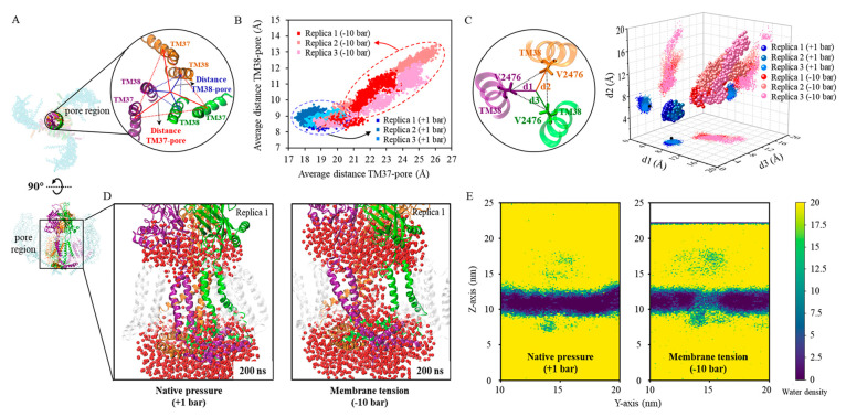
Similar articles
-
Necessity of high-resolution for coarse-grained modeling of flexible proteins.J Comput Chem. 2016 Jul 5;37(18):1725-33. doi: 10.1002/jcc.24391. Epub 2016 Apr 29. J Comput Chem. 2016. PMID: 27130454
-
Separation of time scale and coupling in the motion governed by the coarse-grained and fine degrees of freedom in a polypeptide backbone.J Chem Phys. 2007 Oct 21;127(15):155103. doi: 10.1063/1.2784200. J Chem Phys. 2007. PMID: 17949219
-
Hydration Properties and Solvent Effects for All-Atom Solutes in Polarizable Coarse-Grained Water.J Phys Chem B. 2016 Aug 25;120(33):8102-14. doi: 10.1021/acs.jpcb.6b00399. Epub 2016 Mar 1. J Phys Chem B. 2016. PMID: 26901452 Free PMC article.
-
Modeling Structural Dynamics of Biomolecular Complexes by Coarse-Grained Molecular Simulations.Acc Chem Res. 2015 Dec 15;48(12):3026-35. doi: 10.1021/acs.accounts.5b00338. Epub 2015 Nov 17. Acc Chem Res. 2015. PMID: 26575522 Review.
-
Recent Advances in Coarse-Grained Models for Biomolecules and Their Applications.Int J Mol Sci. 2019 Aug 1;20(15):3774. doi: 10.3390/ijms20153774. Int J Mol Sci. 2019. PMID: 31375023 Free PMC article. Review.
Cited by
-
On the specificity of the recognition of m6A-RNA by YTH reader domains.J Biol Chem. 2024 Dec;300(12):107998. doi: 10.1016/j.jbc.2024.107998. Epub 2024 Nov 17. J Biol Chem. 2024. PMID: 39551145 Free PMC article.
References
MeSH terms
Substances
Grants and funding
LinkOut - more resources
Full Text Sources