Benchmarking informatics approaches for virus discovery: caution is needed when combining in silico identification methods

Abstract

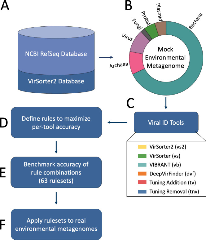
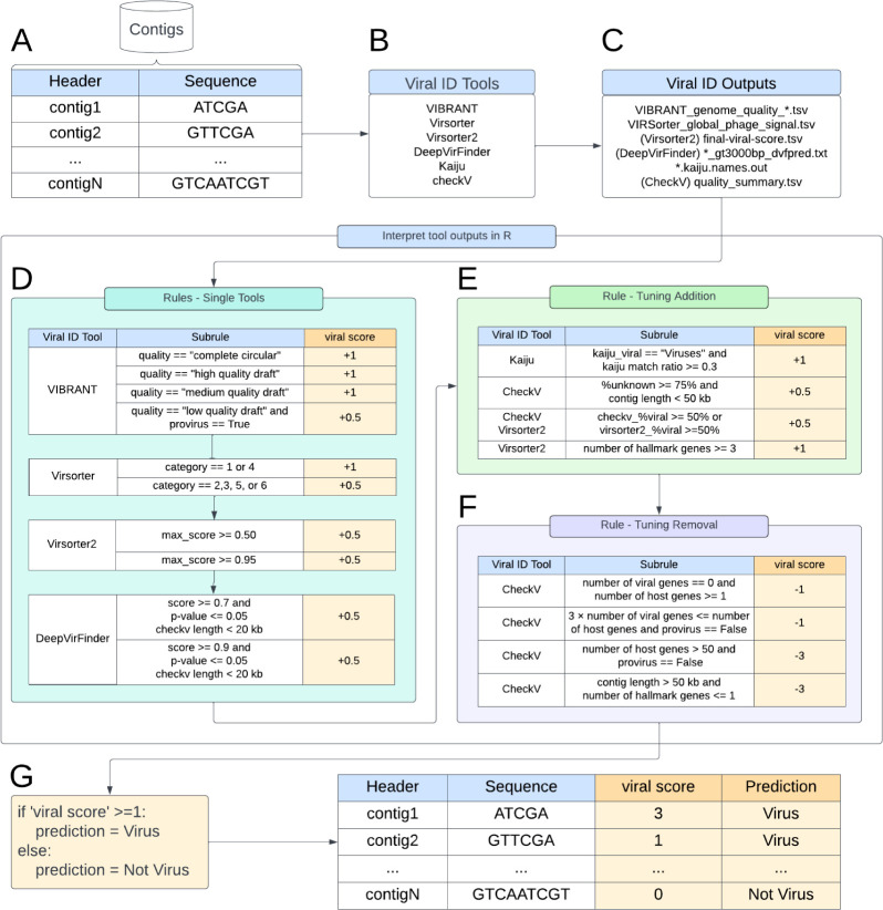
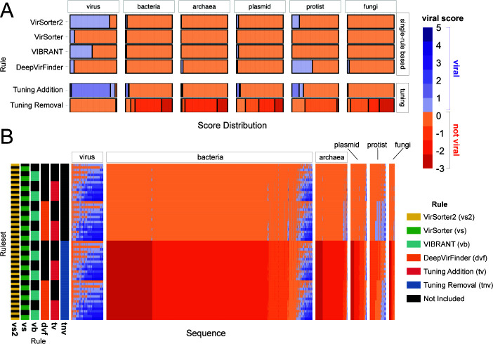
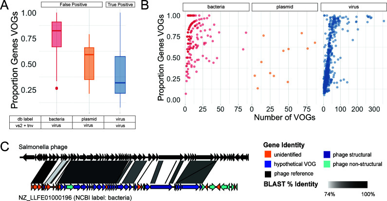
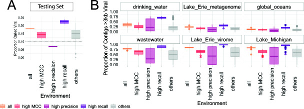
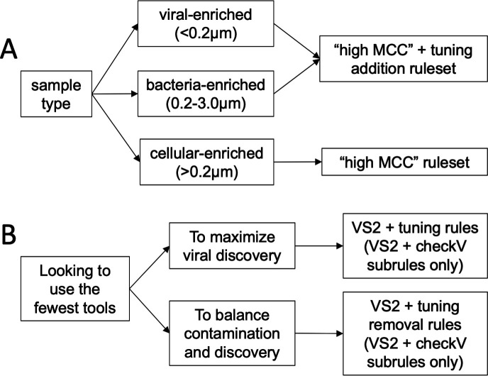
Understanding the ecological impacts of viruses on natural and engineered ecosystems relies on the accurate identification of viral sequences from community sequencing data. To maximize viral recovery from metagenomes, researchers frequently combine viral identification tools. However, the effectiveness of this strategy is unknown. Here, we benchmarked combinations of six widely used informatics tools for viral identification and analysis (VirSorter, VirSorter2, VIBRANT, DeepVirFinder, CheckV, and Kaiju), called "rulesets." Rulesets were tested against mock metagenomes composed of taxonomically diverse sequence types and diverse aquatic metagenomes to assess the effects of the degree of viral enrichment and habitat on tool performance. We found that six rulesets achieved equivalent accuracy [Matthews Correlation Coefficient (MCC) = 0.77, P_adj ≥ 0.05]. Each contained VirSorter2, and five used our "tuning removal" rule designed to remove non-viral contamination. While DeepVirFinder, VIBRANT, and VirSorter were each found once in these high-accuracy rulesets, they were not found in combination with each other: combining tools does not lead to optimal performance. Our validation suggests that the MCC plateau at 0.77 is partly caused by inaccurate labeling within reference sequence databases. In aquatic metagenomes, our highest MCC ruleset identified more viral sequences in virus-enriched (44%-46%) than in cellular metagenomes (7%-19%). While improved algorithms may lead to more accurate viral identification tools, this should be done in tandem with careful curation of sequence databases. We recommend using the VirSorter2 ruleset and our empirically derived tuning removal rule. Our analysis provides insight into methods for in silico viral identification and will enable more robust viral identification from metagenomic data sets.

Importance: The identification of viruses from environmental metagenomes using informatics tools has offered critical insights in microbial ecology. However, it remains difficult for researchers to know which tools optimize viral recovery for their specific study. In an attempt to recover more viruses, studies are increasingly combining the outputs from multiple tools without validating this approach. After benchmarking combinations of six viral identification tools against mock metagenomes and environmental samples, we found that these tools should only be combined cautiously. Two to four tool combinations maximized viral recovery and minimized non-viral contamination compared with either the single-tool or the five- to six-tool ones. By providing a rigorous overview of the behavior of in silico viral identification strategies and a pipeline to replicate our process, our findings guide the use of existing viral identification tools and offer a blueprint for feature engineering of new tools that will lead to higher-confidence viral discovery in microbiome studies.

Keywords: bacteriophages; metagenomics; microbial ecology; viral discovery.

Fig 1

Overview of study workflow. (A) A set of sequences > 3 kb were randomly downloaded from NCBI and a curated Non-RefSeq viral genomes database (“VirSorter2 database”) to (B) generate five mock environmental metagenomes, where the donut chart represents the proportion of each sequence type in each mock metagenome. (C) Mock metagenomes were run through six viral identification tools, (D) where score cutoffs were defined based on each tool’s outputs to maximize their accuracy. (E) Accuracy was then assessed for each tool combination to guide the development of defined “rulesets.” (F) Rulesets were then used to classify sequences from six real-world aquatic metagenomes: three cell-enriched metagenomes and three virus-enriched metagenomes.

Fig 2

Diagram of approach details. (A) Sequences are first processed by each (B) viral identification tool. Next, (C) the tool outputs are programmatically post-processed to generate a viral score based on both (D) single-tool rules and the data-driven creation of (E) tuning addition and (F) tuning removal processes. (G) This combined post-processing generates a viral score that indicates whether each sequence input is predicted as “Virus” or “Not Virus.” Subrules are scored based on the confidence of the prediction: low confidence = ±0.5, confident = ±1, and highly confident not viral = −3.

Fig 3

Comparison of different rulesets. (A) Distribution of viral scores assigned to mock metagenome sequences for our six rules: four single-tool and two tuning rules. (B) Viral scores of all sequences across six mock metagenomes classified by each ruleset. Ruleset rows are colored based on whether or not each rule was used to attain the viral score result for a given sequence. In both A and B, viral scores ≥ 1 are classified as viral and <1 as not viral. All sequences are grouped by their assigned taxonomy.

Fig 4

Performance of the 63 rulesets. (A) Box and whisker plots of the performance scores representing variation in MCC, precision, and recall of different rulesets based on the number of rules used for prediction. (B) Ruleset accuracy (MCC) ordered by increasing MCC and colored based on the ruleset’s type according to statistically equivalent (P_adj ≥ 0.05) rulesets. For A and B, the middle line represents the group mean; boxes above and below the middle line represent the top and bottom quartiles, respectively; whiskers above and below the boxes represent 1.5 times the interquartile range (roughly the 95% CI), outliers are represented by circles beyond the whiskers. The boxplots in A are overlaid with points that represent each testing set’s MCC.

Fig 5

Proportion of viruses in common between rulesets. Heatmap values calculated by dividing the intersection (called viral by both rulesets) by the union (called viral by at least one) of the viruses found by both rulesets, which represents the proportion in common between the tools (scale bar on right: dark-purple: 0–0.1, blue: 0.1–0.5, green: 0.5–0.9, and yellow: 0.9–1). The bar to the left of the heatmap represents the total number of viruses identified by each tool combination (scalebar to its left). The bars above the heatmap indicate the tool(s) used in the rulesets, as well as the ruleset type.

Fig 6

Mislabeled sequences. (A) Box and whisker plots of the proportion of genes on a sequence with a VOG annotation by VIBRANT broken down by sequence type (for the high-MCC rules). (B) Proportion of a sequence’s genes with a VOG annotation versus the number of genes with a VOG annotation faceted by sequence type. Because VIBRANT is the only tool that provided VOG annotation, only sequences classified as viral by VIBRANT are included in panels A and B (which only included bacteria, viruses, and plasmids). (C) Sequence synteny plots indicating sequence similarity between a representative bacterial “false positive:” NZ_LLFE01000196 (NCBI label: bacteria) versus Salmonella phage SSU5. All genes of the testing set sequences are colored by their gene identity.

Fig 7

Proportion of viruses predicted by each tool combination across (A) our testing sets and (B) environmental data sets. Rulesets are grouped based on the accuracy type on the testing set shown in the highlighted rulesets in Fig. 5.

Fig 8

Recommendations. Flowcharts are based on (A) sample type and (B) study goals when looking to minimize the number of tools used.

References

1. Guidi L, Chaffron S, Bittner L, Eveillard D, Larhlimi A, Roux S, Darzi Y, Audic S, Berline L, Brum J, et al. . 2016. Plankton networks driving carbon export in the oligotrophic ocean. Nature 532:465–470. doi:10.1038/nature16942 - DOI - PMC - PubMed
1. Wilhelm SW, Suttle CA. 1999. Viruses and nutrient cycles in the sea: viruses play critical roles in the structure and function of aquatic food webs. BioScience 49:781–788. 10.2307/1313569. - DOI
1. Howard-Varona C, Lindback MM, Bastien GE, Solonenko N, Zayed AA, Jang H, Andreopoulos B, Brewer HM, Glavina Del Rio T, Adkins JN, Paul S, Sullivan MB, Duhaime MB. 2020. Phage-specific metabolic reprogramming of virocells. ISME J 14:881–895. doi:10.1038/s41396-019-0580-z - DOI - PMC - PubMed
1. Hurwitz BL, U’Ren JM. 2016. Viral metabolic reprogramming in marine ecosystems. Curr Opin Microbiol 31:161–168. doi:10.1016/j.mib.2016.04.002 - DOI - PubMed
1. Beumer A, Robinson JB. 2005. A broad-host-range, generalized transducing phage (SN-T) acquires 16S RRNA genes from different genera of bacteria. Appl Environ Microbiol 71:8301–8304. doi:10.1128/AEM.71.12.8301-8304.2005 - DOI - PMC - PubMed
LinkOut - more resources