Inhibition of cysteine protease disturbs the topological relationship between bone resorption and formation in vitro

Abstract

Introduction: Osteoporosis is a global health issue. Bisphosphonates that are commonly used to treat osteoporosis suppress both bone resorption and subsequent bone formation. Inhibition of cathepsin K, a cysteine proteinase secreted by osteoclasts, was reported to suppress bone resorption while preserving or increasing bone formation. Analyses of the different effects of antiresorptive reagents such as bisphosphonates and cysteine proteinase inhibitors will contribute to the understanding of the mechanisms underlying bone remodeling.

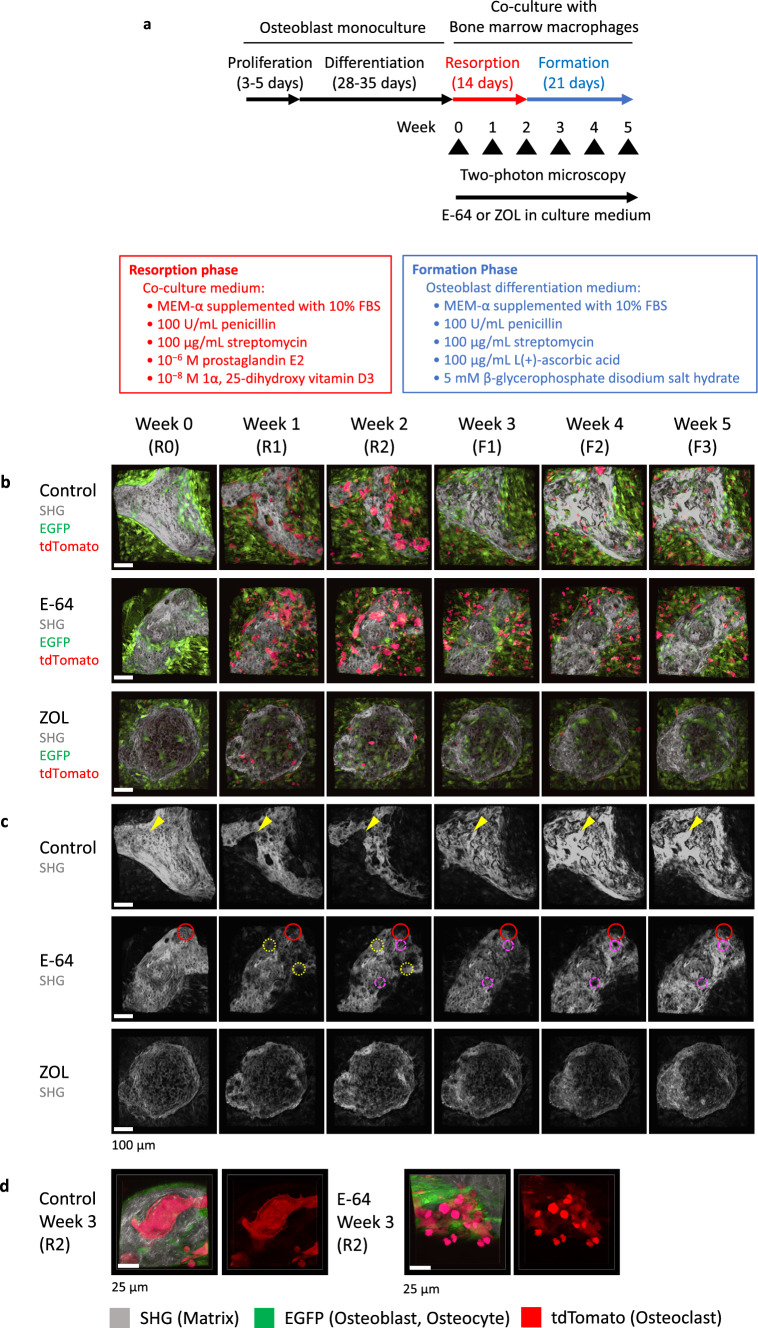
Materials and methods: Our team has developed an in vitro system in which bone remodeling can be temporally observed at the cellular level by 2-photon microscopy. We used this system in the present study to examine the effects of the cysteine proteinase inhibitor E-64 and those of zoledronic acid on bone remodeling.

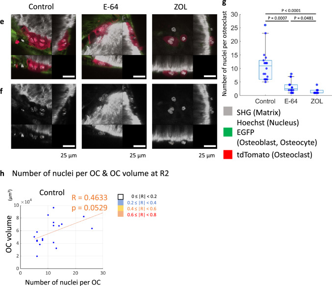
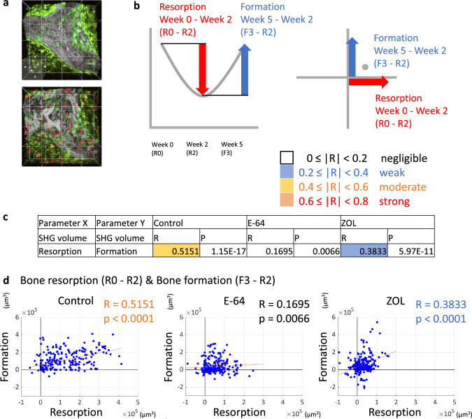
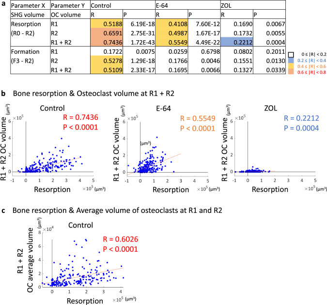
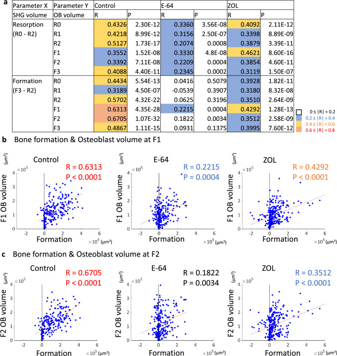
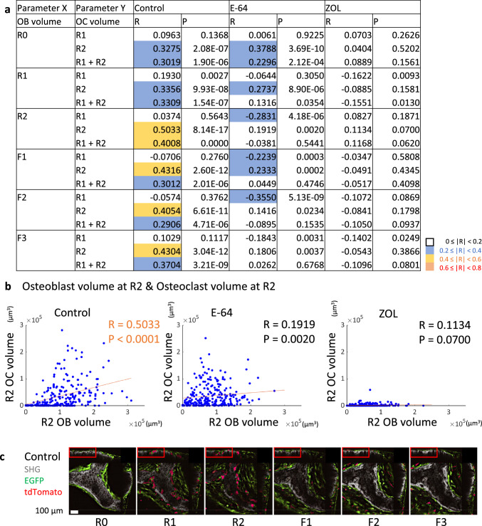
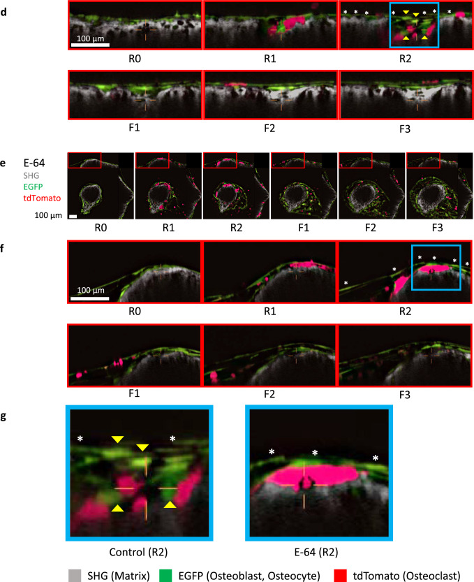
Results: In the control group, the amount of the reduction and the increase in the matrix were correlated in each region of interest, indicating the topological and quantitative coordination of bone resorption and formation. Parameters for osteoblasts, osteoclasts, and matrix resorption/formation were also correlated. E-64 disrupted the correlation between resorption and formation by potentially inhibiting the emergence of spherical osteoblasts, which are speculated to be reversal cells in the resorption sites.

Conclusion: These new findings help clarify coupling mechanisms and will contribute to the development of new drugs for osteoporosis.

Keywords: Bone remodeling; Cathepsin K; Coupling; Osteoblast; Osteoclast; Two-photon microscopy.

Fig. 1

The in vitro reconstitution system of bone remodeling. a Schema of the experimental design. Weeks 0, 1, 2, 3, 4, and 5 are referred to as R0, R1, R2, F1, F2, and F3 hereafter. b, c Volumetric views of 3D data acquired by 2-photon microscopy. Maximal impression images shown by IMARIS are presented. b Volumetric views of all channels. Gray: second harmonic generation (SHG; collagen). Green: EGFP (osteoblasts). Red: tdTomato (osteoclasts). c Volumetric views of the SHG channel. To make the images more visible, the brightness of each image was modified using look-up tables (LUTs) and the same values. Scale bar: 100 µm. Yellow arrowheads in the control group: representative resorption pits that were filled with the new matrix created. Dotted yellow circles in E-64: sites at which resorption occurred in the 1st week of the resorption phase and formation occurred in the 2nd week. Dashed magenta circles in E-64: sites at which formation occurred in the 1st week of the formation period, resorption occurred in the 2nd week, and formation occurred again in the 3rd week. d Zoom-up images of osteoclasts shown by NIS-elements AR software (Nikon). e, f Orthogonal views of osteoclasts at R2. The nuclei were stained with Hoechst 33342. The images are via NIS-elements AR. Scale bar: 25 µm. e Volumetric views of all channels. Gray: SHG. Green: EGFP (osteoblasts). Red: tdTomato (osteoclasts). f Volumetric views of the SHG channel. g Quantification of the number of nuclei per osteoclast in panels e and f. Data were analyzed by the Kruskal–Wallis test followed by the Steel–Dwass test. Six fields of each dish were observed, and the experiment was carried out three times (n = 18). Data are mean ± SE. h A scatterplot between the number of nuclei per osteoclast and the osteoclast volume (R2). Spearman’s rank correlation coefficients (R) and p values. n = 18

Fig. 1

The in vitro reconstitution system of bone remodeling. a Schema of the experimental design. Weeks 0, 1, 2, 3, 4, and 5 are referred to as R0, R1, R2, F1, F2, and F3 hereafter. b, c Volumetric views of 3D data acquired by 2-photon microscopy. Maximal impression images shown by IMARIS are presented. b Volumetric views of all channels. Gray: second harmonic generation (SHG; collagen). Green: EGFP (osteoblasts). Red: tdTomato (osteoclasts). c Volumetric views of the SHG channel. To make the images more visible, the brightness of each image was modified using look-up tables (LUTs) and the same values. Scale bar: 100 µm. Yellow arrowheads in the control group: representative resorption pits that were filled with the new matrix created. Dotted yellow circles in E-64: sites at which resorption occurred in the 1st week of the resorption phase and formation occurred in the 2nd week. Dashed magenta circles in E-64: sites at which formation occurred in the 1st week of the formation period, resorption occurred in the 2nd week, and formation occurred again in the 3rd week. d Zoom-up images of osteoclasts shown by NIS-elements AR software (Nikon). e, f Orthogonal views of osteoclasts at R2. The nuclei were stained with Hoechst 33342. The images are via NIS-elements AR. Scale bar: 25 µm. e Volumetric views of all channels. Gray: SHG. Green: EGFP (osteoblasts). Red: tdTomato (osteoclasts). f Volumetric views of the SHG channel. g Quantification of the number of nuclei per osteoclast in panels e and f. Data were analyzed by the Kruskal–Wallis test followed by the Steel–Dwass test. Six fields of each dish were observed, and the experiment was carried out three times (n = 18). Data are mean ± SE. h A scatterplot between the number of nuclei per osteoclast and the osteoclast volume (R2). Spearman’s rank correlation coefficients (R) and p values. n = 18

Fig. 2

Analyses of SHG, tdTomato, and EGFP volumes. a Surface rendering of the SHG positive area (upper panel). The value of the area of maximum SHG projection at week 0 (lower panel) was used to adjust the SHG volumes. Temporal changes in the SHG (b), tdTomato (d), and EGFP (f) volume for each group. Data are mean ± SE. The Friedman test followed by Bonferroni adjustment was used to determine the significance of differences between the values at each time point. c, e, g Comparisons of the three groups’ values at each time point. Data are mean ± SE and were analyzed by the Kruskal–Wallis test followed by the Steel–Dwass test. Control: n = 15, E-64: n = 16, ZOL: n = 17. c SHG, e tdTomato, g EGFP

Fig. 2

Analyses of SHG, tdTomato, and EGFP volumes. a Surface rendering of the SHG positive area (upper panel). The value of the area of maximum SHG projection at week 0 (lower panel) was used to adjust the SHG volumes. Temporal changes in the SHG (b), tdTomato (d), and EGFP (f) volume for each group. Data are mean ± SE. The Friedman test followed by Bonferroni adjustment was used to determine the significance of differences between the values at each time point. c, e, g Comparisons of the three groups’ values at each time point. Data are mean ± SE and were analyzed by the Kruskal–Wallis test followed by the Steel–Dwass test. Control: n = 15, E-64: n = 16, ZOL: n = 17. c SHG, e tdTomato, g EGFP

Fig. 2

Analyses of SHG, tdTomato, and EGFP volumes. a Surface rendering of the SHG positive area (upper panel). The value of the area of maximum SHG projection at week 0 (lower panel) was used to adjust the SHG volumes. Temporal changes in the SHG (b), tdTomato (d), and EGFP (f) volume for each group. Data are mean ± SE. The Friedman test followed by Bonferroni adjustment was used to determine the significance of differences between the values at each time point. c, e, g Comparisons of the three groups’ values at each time point. Data are mean ± SE and were analyzed by the Kruskal–Wallis test followed by the Steel–Dwass test. Control: n = 15, E-64: n = 16, ZOL: n = 17. c SHG, e tdTomato, g EGFP

Fig. 3

Analysis of regional changes in the SHG volume. a Sixteen regions of interest (ROIs) in one field of view. b Explanatory diagrams for the values of bone resorption and bone formation, and the scatterplots. Changes in the values during the resorption phase (week 0 [R0] to week 2 [R2]) and the formation phase (week 2 [R2] to week 5 [F3]) are plotted. c, d Spearman’s rank correlation coefficients (R) and p values (c) and scatterplots (d) for bone resorption and bone formation. Control: n = 240, E-64: n = 256, ZOL: n = 272

Fig. 4

Analysis of the correlations between the matrix changes and the osteoclast volume. a Correlations between the changes in the matrix volume and the changes in the osteoclast volume. Spearman’s rank correlation coefficients (R) and p values. b Scatterplots between bone resorption and the cumulative osteoclast volume (R1 + R2). Control: n = 240, E-64: n = 256, ZOL: n = 272. c A scatterplot between bone resorption and the total volume of osteoclasts with a volume over 2000 µm² at R1 and R2, divided by the number of ROI. Spearman’s rank correlation coefficients (R) and p values. Control: n = 240

Fig. 5

Analysis of the correlations between matrix changes and the EGFP volume. a Correlations between bone resorption/formation and the osteoblast volume. Spearman’s rank correlation coefficients (R) and p values are presented. b, c Scatterplots between bone formation and the osteoblast volume at F1 (b), and F2 (c). Control: n = 240, E-64: n = 256, ZOL: n = 272

Fig. 6

Analysis of the correlations between bone resorption/formation and osteoblast sphericity. a Surface rendering of SHG and EGFP shown by the Imaris software. The EGFP-positive area is shown with a heatmap indicating the extent of sphericity. Scale bar: 100 µm. b Correlations between bone formation/resorption and osteoblast sphericity. Spearman’s rank correlation coefficients (R) and p values are presented. c Scatterplots between bone formation and the osteoblast sphericity at R2. Control: n = 240, E-64: n = 256, ZOL: n = 272

Fig. 7

Analysis of the correlations between the osteoblast volume and osteoclast volume. a Correlations between the osteoblast volume and osteoclast volume. Spearman’s rank correlation coefficients (R) and p values are presented. b Scatterplots between the osteoblast volume at R2. Control: n = 240, E-64: n = 256, ZOL: n = 272. c–g Orthogonal views of resorption pits in the control and E-64 groups. c Orthogonal views of the control (see Fig. 1b). The images were revealed by NIS-elements AR software. d Cropped pictures of panel c are indicated by red boxes. Yellow arrowheads: spherical osteoblasts. *Flat osteoblasts. e Orthogonal views of E-64 (see Fig. 1b). The images are by NIS-elements AR. f Cropped pictures of panel e are indicated by red boxes. *Flat osteoblasts. To make images more visible, the brightness of each image was modified using LUTs and the same values. Scale bar: 100 µm. g Cropped pictures of panels d and f, respectively, as indicated by blue boxes. Yellow arrowheads: spherical osteoblasts. *Flat osteoblasts

Fig. 7

Analysis of the correlations between the osteoblast volume and osteoclast volume. a Correlations between the osteoblast volume and osteoclast volume. Spearman’s rank correlation coefficients (R) and p values are presented. b Scatterplots between the osteoblast volume at R2. Control: n = 240, E-64: n = 256, ZOL: n = 272. c–g Orthogonal views of resorption pits in the control and E-64 groups. c Orthogonal views of the control (see Fig. 1b). The images were revealed by NIS-elements AR software. d Cropped pictures of panel c are indicated by red boxes. Yellow arrowheads: spherical osteoblasts. *Flat osteoblasts. e Orthogonal views of E-64 (see Fig. 1b). The images are by NIS-elements AR. f Cropped pictures of panel e are indicated by red boxes. *Flat osteoblasts. To make images more visible, the brightness of each image was modified using LUTs and the same values. Scale bar: 100 µm. g Cropped pictures of panels d and f, respectively, as indicated by blue boxes. Yellow arrowheads: spherical osteoblasts. *Flat osteoblasts

References

1. Holroyd C, Cooper C, Dennison E. Epidemiology of osteoporosis. Best Pract Res Clin Endocrinol Metab. 2008;22:671–685. doi: 10.1016/j.beem.2008.06.001. - DOI - PubMed
1. Klibanski A, Adams-Campbell L, Bassford T, et al. Osteoporosis prevention, diagnosis, and therapy. J Am Med Assoc. 2001;285:785–795. doi: 10.1001/jama.285.6.785. - DOI
1. Reid IR, Billington EO. Drug therapy for osteoporosis in older adults. Lancet. 2022;399:1080–1092. doi: 10.1016/S0140-6736(21)02646-5. - DOI - PubMed
1. Bone HG, Hosking D, Devogelaer J-P, et al. Ten years’ experience with alendronate for osteoporosis in postmenopausal women. N Engl J Med. 2004;350:1189–1199. doi: 10.1056/NEJMoa030897. - DOI - PubMed
1. Unnanuntana A, Rebolledo BJ, Michael Khair M, et al. Diseases affecting bone quality: beyond osteoporosis. Clin Orthop Relat Res. 2011;469:2194–2206. doi: 10.1007/s11999-010-1694-9. - DOI - PMC - PubMed