. 2024 Feb 20;20(2):e1011839.
doi: 10.1371/journal.pcbi.1011839. eCollection 2024 Feb.

Fast adaptation to rule switching using neuronal surprise

Affiliations

Fast adaptation to rule switching using neuronal surprise

Martin L L R Barry et al. PLoS Comput Biol. .

Abstract

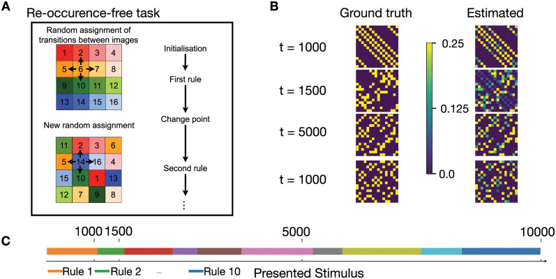
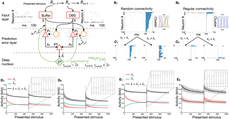
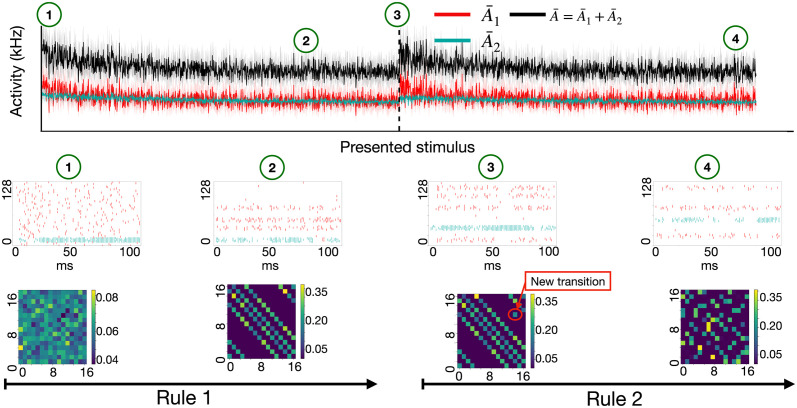
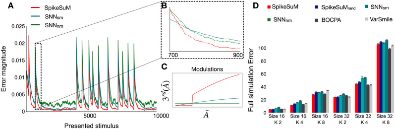
In humans and animals, surprise is a physiological reaction to an unexpected event, but how surprise can be linked to plausible models of neuronal activity is an open problem. We propose a self-supervised spiking neural network model where a surprise signal is extracted from an increase in neural activity after an imbalance of excitation and inhibition. The surprise signal modulates synaptic plasticity via a three-factor learning rule which increases plasticity at moments of surprise. The surprise signal remains small when transitions between sensory events follow a previously learned rule but increases immediately after rule switching. In a spiking network with several modules, previously learned rules are protected against overwriting, as long as the number of modules is larger than the total number of rules-making a step towards solving the stability-plasticity dilemma in neuroscience. Our model relates the subjective notion of surprise to specific predictions on the circuit level.


Conflict of interest statement

The authors have declared that no competing interests exist.

Figures

Fig 1
Fig 1. Expected transitions in a volatile sequence task.
A. At each presentation step, the stimulus presents the wallpaper image (indicated by different colors) in one of the rooms of an apartment with R rooms (here R=16). The stimulation sequence reflects transitions (arrows) from the current room (current image) to one of the K neighboring rooms (here K = 4). On rare occasions (change points), the transition rule is changed by a new random assignment of images to rooms. The same rule is unlikely to return. B. The ground truth transition matrix Ti,j*(m) for different rules m = 1, … 4 (left, yellow indicates Ti,j*=1/4, dark blue Ti,j*=0), compared to the transition matrix Tij estimated by the model (right, light blue and green: 0 < Tij < 1/4) at different time points of a simulation run. Rule 1 at t = 1000 corresponds to the first configuration in A. C. Switching of rules over time in the simulation of B. Each rule (Rule 1, Rule 2, …) only appears once. Vertical lines indicate the time points in B.
Fig 2
Fig 2. Neurons in prediction error layer respond to unexpected transitions.
A. Spiking network model ‘SpikeSuM’. From top to bottom: Every 100ms stimuli change, giving rise to a sequence Rn−1, Rn, Rn+1… The presently observed stimulus (Rn, red box ‘OBS’) and the previous stimulus (Rn−1, ‘Buffer’) are encoded with spike trains of 128 neurons each (16 sample spike trains shown). These spike trains are transmitted to two excitation-inhibition networks (prediction error layer) composed of pyramidal neurons (red triangles) and inhibitory neurons (orange circles). Pyramidal neurons in population P1 are excited (arrowheads) by the inputs representing the prediction X^ based on stimulus Rn−1 and inhibited (round heads) by the current observation X whereas neurons in P2 are inhibited by the prediction X^ and excited by the current observation X. The activity A1 and A2 of populations P1 and P2 is transmitted to pyramidal tract neurons (PT), which low-pass filter the activity and transmit it to a group of neurons in a deep nucleus (green, labeled 3rd) which sends a neuromodulatory surprise signal back to the prediction error layer. Poorly predicted stimuli increase activity in the prediction error layer and indirectly accelerate, via the 3rd factor, learning in the plastic connections (red lines). Inset: Time course of the 3rd factor (green) over 4s before and after a rule switch at time tswitch. B: Spike trains of all 128 pyramidal neurons in population P2 during a specific stimulus Rn. The 128 neurons have first been ordered from highest to lowest firing rate and then clustered into groups of 8 neurons, with neurons 1 to 8 forming the first cluster. Right: Histogram of average firing rate per cluster (horizontal bars). B1: Random sparse connectivity from presynaptic neurons in the input layer to neurons in the prediction error layer. Inset: schematics, colors indicate connection strength from red (weak) to blue (strong). B2: Regular connectivity with binary connections. Inset: schematics, nonzero connections (blue) are organized in clusters of 8 neurons, but for readability, only 4 clusters of two neurons each are shown. C1 and C2: To compare the two networks, we show the spikes generated in response to a new stimulus Rn while keeping the same order of neurons. For random connectivity (C1) spike plots are different if RnRn but similar if Rn = Rn. The same holds for regular connectivity (C2). D1 and D2: Filtered activity of pyramidal neurons in populations P1 (red), P2 (cyan), and the total filtered activity A¯ (black) as a function of time-averaged over 100 different sequences with a change point (switch of rule) after 500 presentation steps, for random (D1) or regular (D2) connectivity (parameter K = 2). Both networks indicate a surprising transition (dashed vertical line) by increased activity. Insets show the activity before and after the rule switch. E1 and E2: Same as in D1 and D2, but for the case of K = 4 possible next stimuli. Since predictions are less reliable, the activity A¯ converges to higher levels.
Fig 3
Fig 3. Neuronal responses depend on the present stimulus, the previous stimulus, and consistent alternatives to the present stimulus in a task with R=16 stimuli and K = 4 transitions possibilities and two rules.
Top: Activity (arbitrary units) of populations P1 (green) and P2 (red) as well as the total activity A¯ (black) of all pyramidal neurons. After 1500 presentation steps, the transition rule switches from rule 1 to rule 2. Each presentation step corresponds to the exposure to one stimulus for 100ms. Middle: Spike trains of pyramidal neurons during one presentation step, at different points during learning (from left to right): at the beginning (label 1) and end of the first episode with rule 1 (label 2) and beginning (label 3) and end of the first episode with rule 2 (label 4). If the observation is stronger than the prediction neurons in population P2 fire (blue dots); whereas if the observation is weaker than the prediction neurons in population P1 fire (red dots). Pyramidal neurons (16 per stimulus, 8 neurons each from P1 and P2) have been sorted according to stimulus numbers for visual clarity. Bottom. Matrix of transitions between stimuli decoded from the weights onto pyramidal neurons. At the end of the first presentation step after a change point (label 3), a new element (red arrow) has appeared in the transition matrix corresponding to the newly observed transition, Rn−1Rn. After some time with the novel rule, the new transition matrix is learned (label 4) and the old one is suppressed.
Fig 4
Fig 4. Rapid adaptation enabled by surprise-modulated three-factor plasticity.
A: Error magnitude of the transition matrix (Frobenius norm between the true transition matrix T* and the estimated matrix T) as a function of time for the SpikeSuM model (red), and a Spiking Neural Network model (SNN) with the same architecture and number of neurons as SpikeSuM, but simple modulation (cyan SNNsm) or no modulation (green SNNnm), in a volatile sequence task with R=16 different stimuli and K = 4 possible transitions. Rule switches cause the occasional abrupt increases in error. The SpikeSuM network exhibits faster learning immediately after the switch as well as better convergence during periods when the rule stays fixed; volatility H=0.001. B Zoom on 200 presentation steps immediately after a rule switch. The red curve goes down faster and to a lower value than the other two. C: The surprise signal transmitted by the 3rd factor as a function of the activity A¯ for three cases (red: SpikeSuM rule; cyan: simplified modulation rule; green: constant learning rate, no modulation). The parameters of all three rules have been optimized. D Average error over 10’000 presentation steps with volatility H = 0.001 for different values of R (size) and K. The performance of SpikeSuM is comparable to that of the Bayesian Online Change Point detection algorithm (BOCPA, black) and varSMile (grey) and better than SNNnm or SNNsm. The results with random connectivity SpikeSuMrand are shown in dark blue.
Fig 5
Fig 5. Behavioral surprise of human participants compared to simulated surprise.
Example of an image sequence. Each image is presented for 1s followed by a 1s grey screen. Subjects are informed to focus on one specific image (e.g. ‘pen’) and the transition from there to the following image. B Sequence 1 is deterministic and used to familiarize the subject with the task. Sequence 2 has stochastic transitions so that each given image can be followed by one of K = 2 other images, with equal probability p = 0.5. C Participants observe the image sequence while attempting to predict the image following the pen and report their feeling of surprise continuously by moving a ‘Surprise slider’. Participants are randomly assigned to two different groups, with and without change points. D Scaled normalized surprise S^ reported by the 65 participants in group 1 (blue line: mean; shaded blue: variance) as a function of time (Methods), overlaid with appropriately scaled surprise in 60 simulations with SpikeSuM (green line: mean; shaded green: variance) using the same sequence as in the experiments with change point after 150 image presentations. E Same as D, but for the sequence without change-points. F Differences in the experimental data of participants are significant (t-test) in D between the 50 steps before and 50 steps after the change point (blue bars in F); not significant in E between the 50 steps before and 50 steps after step 150 in the absence of change point; and significant for the time steps 150–200 between D and E (blue vs. red bar in F). The symbol *** indicates p < 10−5, and ‘ns’ not significant.
Fig 6
Fig 6. Continual learning across re-occurring rule switches.
A: The SpikeSuM-C network is composed of four layers. The input layer receives the stimulus and connects to the prediction-error layer which is composed of several SpikeSuM modules (cf. Fig 2). A set of context selector modules (CSM) composed of dis-inhibitory networks is bidirectionally connected with the prediction-error layer. Each SpikeSuM module excites its corresponding CSM. A Winner-Take-All circuit in the CSM layer selects the least excited module. Inhibitory feedback weights from the CSM to the prediction-error layer inhibit the PT neurons of unselected SpikeSuM modules, but not the prediction-error neurons (see Material and methods). Red weights are plastic. Non-plastic weights are shown in black for feedforward, solid blue for feedback, and dashed blue for lateral inhibitory connections. B: Connectivity (schematic) within a single module. Disinhibition combined with WTA dynamics selects the module with the lowest activity in the prediction error layer. C: Sequence of rule switches as a function of time. D: Summed activity of all PT-cells (grey, arbitrary units) in a SpikeSuM-C network with 5 modules and error magnitude (green, mismatch between transition matrix in currently selected module and ground truth) during learning. When the second rule appears for the second time, the error exhibits a short spike (green triangle) indicating successful switching between modules. At rare moments (green star marks one of the examples) module switching is initiated at an inappropriate moment but stops immediately thereafter. The activity generated by the switch to an unknown rule is stronger (grey bars exceed the horizontal orange dashed line) than that of a previously observed one (grey bars barely reach the cyan dashed line). Red line: behavior of SpikeSuM (control, 1 single module). E Evolution of synaptic weight matrices over time for each of the five modules. After 500 time steps, the transition matrix of rule 1 has been stored in module 5, and transition matrices of other rules are added as they appear.
Fig 7
Fig 7. Synaptic plasticity as a function of prediction error has two regimes in SpikeSuM-C.
A1-A2: The magnitude of modulation (3rd factor) is shown as a function of the total activity A¯ of layer-2/3 neurons for a SpikeSuM-C network with a single module (A1; equivalent to the original SpikeSuM) and for a SpikeSuM-C network with three modules (A2). The threshold θ is defined in Eq 14. Bars: standard error of the mean. The difference between the two curves (A1-A2) arises from the inhibition of model PT-neurons if they are not located in the winning module: in A1, the activity A¯ of PT neurons always reflects the activity A of layer-2/3 neurons, in A2 it does not. Inset: Histogram of modulation amplitudes 3rd(A¯m) for values slightly above θ: the distribution of modulation amplitudes is bimodal with rare events of large modulation. Arrow: the peak is due to known transitions that remain after a rule change. B1-B2: The update magnitude |Δwik| of a specific synapse is shown as a function of the Hebbian drive Retanh(hi)·EPSC¯k i.e., the multiplication of postsynaptic membrane potential and the current influx caused by presynaptic spike arrival (long-dashed line, averaged over all neurons i in the postsynaptic population P1). Analogously, for postsynaptic population P2 (dotted line) and mean over both populations (solid line). C1-C2: The total amount of synaptic plasticity, represented by the update magnitude ∑kwik| summed over all synapses onto an arbitrary neuron i is shown as a function of the prediction error, represented by the rectified and scaled membrane potential Retanhhi. In a network with a single module (C1), plasticity increases with prediction error so that large prediction errors after a context change lead to overwriting of existing memories. In the network with multiple modules (C2), the plasticity in the SpikeSum-C network exhibits two regimes: prediction errors between 0.1 and 0.4 generate small but non-negligible changes, and induce a refinement of existing memories, whereas for prediction errors above 0.6 existing memories are protected since other memories are created or changed. The error bars represent the 90% confidence interval of the mean. The vertical bar indicates the separation between the two regimes predicted by Gershman et al. [35].
Fig 8
Fig 8. Spike Response Model of neurons in the prediction error layer.
Each postsynaptic neuron receives an input current Ii. This current is integrated, with membrane time constant τ, to obtain the input potential hi. The actual membrane potential of the neuron ui is the combination of both the input potential and a refractory function η, where η is a strong negative potential activated after a spike, forcing the neuron to stay silent for a while. The spike times are then randomly drawn with probability ϕ(ui) generating the spike train of neuron i.
Fig 9
Fig 9. Context selector module (CSM).
Each CSM contains two layers of inhibitory neurons. Layer 1 receives excitatory input from the corresponding SpikeSuM module. Layer 2 receives inhibition from layer 1 and lateral inhibition from layer 2 of other CSMs. The more excitation a CSM receives, the lower the activity in layer 2. Because of WTA dynamics implemented by lateral inhibition, the CSM module with the lowest excitation is selected, inhibits other CSMs, and shuts down the plasticity of other SpikeSuM modules. The red weights are plastic and can be interpreted as a ‘commitment’ to the selected module. The network activity represents the activity across all SpikeSuM modules and supports the WTA dynamics.

Similar articles

Cited by

References

    1. Squires KC, Wickens C, Squires NK, Donchin E. The effect of stimulus sequence on the waveform of the cortical event-related potential. Science. 1976;193:1141–1146. doi: 10.1126/science.959831 - DOI - PubMed
    1. Meyer WU, Niepel M, Rudolph U, Schützwohl A. An experimental analysis of surprise. Cognition & Emotion. 1991;5(4):295–311. doi: 10.1080/02699939108411042 - DOI
    1. Hurley MM, Dennett DC, Adams RB. Inside jokes: Using humor to reverse-engineer the mind. MIT Press, Cambridge; 2011.
    1. Modirshanechi A, Brea J, Gerstner W. A taxonomy of surprise definitions. J Mathem Psychol. 2022;110:102712. doi: 10.1016/j.jmp.2022.102712 - DOI
    1. Schnupp J, Nelken I, King AJ. Auditory Neuroscience: Making Sense of Sound. Cambridge, Mass. (USA): MIT Press; 2011.