Synaptic wiring motifs in posterior parietal cortex support decision-making

Abstract

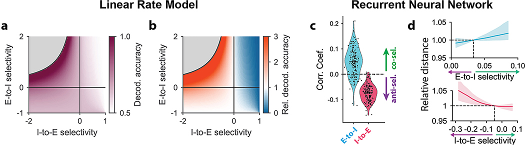
The posterior parietal cortex exhibits choice-selective activity during perceptual decision-making tasks^1-10. However, it is not known how this selective activity arises from the underlying synaptic connectivity. Here we combined virtual-reality behaviour, two-photon calcium imaging, high-throughput electron microscopy and circuit modelling to analyse how synaptic connectivity between neurons in the posterior parietal cortex relates to their selective activity. We found that excitatory pyramidal neurons preferentially target inhibitory interneurons with the same selectivity. In turn, inhibitory interneurons preferentially target pyramidal neurons with opposite selectivity, forming an opponent inhibition motif. This motif was present even between neurons with activity peaks in different task epochs. We developed neural-circuit models of the computations performed by these motifs, and found that opponent inhibition between neural populations with opposite selectivity amplifies selective inputs, thereby improving the encoding of trial-type information. The models also predict that opponent inhibition between neurons with activity peaks in different task epochs contributes to creating choice-specific sequential activity. These results provide evidence for how synaptic connectivity in cortical circuits supports a learned decision-making task.

Extended Data Figure 1:. Trial-type selectivity analysis and image co-registration.

(a) Performance on the navigational two-alternative forced-choice memory task plotted over different daily sessions. Functional data from the last 4 sessions (“late”), which were closest in time to when the brain was preserved for EM, were used for all analyses with the exception of those investigating how structure-function relationships evolve over time (Ext. Data Fig. 5j–k, Ext. Data Fig. 6d), which also include “early” and “middle” sessions. Early, middle, and late sessions were all after the initial training of the animal and comprise expert level task performance. (b) Approximate location of cranial window and calcium imaging ROI relative to cortical regions (adapted from the Allen Mouse Brain Common Coordinate Framework). Although this figure depicts the right hemisphere, the experimental data was collected from the left hemisphere. (c) Calcium imaging ROI: 4 500 μm x 500 μm planes in layer 2/3 (separated by 25 μm in z) were imaged at 5.3 Hz volume rate. (d) Diagram indicating temporal epochs of trial. Different trials were synchronized to temporal landmarks (trial start, cue off, trial end) and 5 temporal trial epochs (cue early, cue late, delay, turn, inter-trial interval (ITI)) were defined relative to those landmarks (Methods). Each epoch lasts 2.2–2.4 seconds. (e) Trial-averaged activity for left (blue) and right (red) trials for several example neurons. Neurons typically have some non-zero activity away from the temporal peak on preferred trial type. (f) Proportion of time points with significant selectivity that share the same trial-type preference as the max selectivity, showing that the left-right direction of max selectivity is generally representative of selectivity throughout the trial, especially for strongly selective neurons. (g) Max selectivity for functionally characterized neurons contained within the EM volume (n = 134 neurons active in the last 4 sessions). (h) Cumulative histograms of mutual information with trial type, demonstrating that it was not statistically different between inhibitory (purple solid line) and excitatory (green solid line) neurons (p = 0.20, K-S test). Shading indicates 95% confidence intervals generated via bootstrap. (i) Corresponding slices from co-registered two-photon calcium imaging (2p, top) and EM (bottom) datasets. Cyan arrows – blood vessels used as landmarks. (j) Example cellular ROIs (green) co-registered to calcium imaging (top) and EM data (bottom).

Extended Data Figure 2:. Trial-averaged neuron activity.

Each row shows trial-averaged activity of a functionally-characterized neuron. Row labels are neuron IDs corresponding to the CATMAID EM database, Extended Data Figures 2 and 3, and Supplementary Tables 1 and 2. Left and right columns show activity on left and right trials, respectively. Temporal epochs shown correspond to Ext. Data Fig. 1d. Activity was averaged over the last 4 behavioral sessions, then normalized by the maximum activity rate over both trial types for each neuron separately. Neurons were sorted first by selectivity (indicated by colored bars on y-axis: left (max selectivity < −0.05) – blue, right (max selectivity > 0.05) – red, non-selective (−0.5 ≤ max selectivity ≤ 0.05) – gray), then by timepoint of maximum mutual information with trial type (early to late).

Extended Data Figure 3:. Excitatory Neuron Morphologies.

Traced neuron morphologies are shown for functionally-characterized excitatory pyramidal neurons in PPC. Axon – blue, dendrites – orange. Labels are neuron IDs corresponding to the CATMAID database and Supplementary Tables 1 and 2. Scale bars: 50 μm.

Extended Data Figure 4:. Inhibitory Neuron Morphologies.

Traced neuron morphologies are shown for functionally-characterized inhibitory neurons in PPC. Axon – blue, dendrites – orange. Labels are neuron IDs corresponding to the CATMAID database and Supplementary Tables 1 and 2. Scale bars: 50 μm.

Extended Data Figure 5:. Co-selective Excitatory-to-Inhibitory Connectivity and Simultaneous-Selectivity Analysis.

(a) Number of synapses plotted as a function of axon/dendrite overlap for E-to-I neuron pairs, including both connected and non-connected pairs. Co-selective pairs (green) generally have more synapses per overlap than anti-selective (purple). Dotted lines indicate linear fits. (b) Normalized synapse frequency for E-to-I connections including non-connected pairs, calculated by pooling all co- or anti-selective pairs together (Methods). Co-selective pairs have higher normalized synapse frequency than anti-selective pairs (anti: 0.0315 ± 0.001 μm⁻¹, n=21 pairs, co: 0.0157 ± 0.001 μm⁻¹, n=21, p < 0.001, bootstrap test). Violin plots show distributions generated via bootstrap. (c) Max-selectivity similarity as a function of the max selectivity of the two neurons. Co-selective neuron pairs have positive (green) and anti-selective pairs have negative values (purple). (d) Correlation coefficient between normalized synapse frequency and selectivity similarity for E-to-I connections in PPC (as in Fig. 2h), calculated using different distance thresholds for determining axon/dendrite overlap (see Fig. 2b). Gray shading indicates correlations expected by chance (95% confidence interval of random shuffles). The correlation is significant over a broad range of values (~2–18) μm, and is maximized for thresholds close to value used (5 μm, dotted line). (e) Top: instantaneous selectivity for example right- (red) and left-selective (blue) neurons. Arrows indicate max selectivity for each neuron. Bottom: simultaneous-selectivity similarity quantifies the selectivity similarity between neurons at the same time point. Arrow indicates the maximum absolute value, which is used for x-axis values in (e) and (f). (f) Simultaneous-selectivity similarity is correlated to connection frequency (n = 21 pairs, r = 0.58, p = 0.006, Pearson correlation test). (g) Simultaneous-selectivity similarity is correlated to synapse size (n = 29 synapses, r = 0.50, p = 0.006, Pearson correlation test). (h) Number of neurons that change max selectivity from left to right or vice versa (“switch”), or keep the same right-left selectivity (“stay”), between early (8–10 days before sacrifice) and late (0–3 days before) sessions. Gray region indicates expected range if neurons switch at chance levels. (i) Number of neuron pairs that change max-selectivity similarity from co- to anti-selective or vice versa (“switch”), or keep the same similarity (“stay”) between early and late sessions. Gray region indicates expected range if neurons switch at chance levels. (j) Correlations between normalized synapse frequency and max-selectivity similarity for E-to-I connections in PPC, calculated using functional data from early (8–10 days before sacrifice), middle (4–7 days before), and late sessions (0–3 days before). Correlation coefficients are lower for earlier sessions (early: r = 0.31, p = 0.27, middle: r = 0.53, p = 0.019, late: r = 0.66, p = 0.001, Pearson correlation tests). (k) Correlations between PSD area and max-selectivity similarity for E-to-I synapses in PPC, calculated for early, middle, and late sessions. Correlation coefficients are lower for earlier sessions (early: r = 0.19, p = 0.42, middle: r = 0.46, p = 0.023, late: r = 0.56, p = 0.002, Pearson correlation tests). All statistics reported as mean ± standard error with two-tailed significance tests.

Extended Data Figure 6:. Anti-selective Inhibitory-to-Excitatory Connectivity and Interneuron Subtype Analysis.

(a) Number of synapses plotted as a function of axon/dendrite overlap for I-to-E neuron pairs, including both connected and non-connected pairs. Anti-selective pairs (purple) generally have more synapses per overlap than co-selective pairs (green). Dotted lines indicate linear fits. (b) Normalized synapse frequency for I-to-E connections including non-connected neuron pairs, calculated by pooling co- or anti-selective pairs together (Methods). Anti-selective pairs have higher normalized synapse frequency than co-selective pairs (anti: 0.0109 ± 0.0004 μm⁻¹, n = 99 pairs, co: 0.0096 ± 0.0003 μm⁻¹, n = 112, p = 0.03, bootstrap test). Violin plots show distributions generated via bootstrap. (c) Correlation coefficient between normalized synapse frequency and selectivity similarity for I-to-E connections (as in Fig. 3c, calculated using different distance thresholds for determining axon/dendrite overlap (see Fig. 2b). Gray shading indicates correlations expected by chance (95% confidence interval of random shuffles). The correlation is significant over a range of values (~3–15 μm), and is maximized for distances thresholds close to value used (5 μm, dotted line). (d) Normalized synapse frequency plotted as a function of max-selectivity similarity for I-to-E connections in PPC, calculated using functional data from early (8–10 days before sacrifice), middle (4–7 days before), and late (0–3 days before) sessions. Correlation coefficients are less negative for earlier sessions (early: r = −0.06, p = 0.52; middle: r = −0.05, p = 0.64; late: r = −0.22, p = 0.021, Pearson correlation test). (e) Simultaneous-selectivity similarity is negatively correlated to normalized synapse frequency (r = −0.20, p = 0.041, Pearson correlation test). (f-m): Structure-function correlations for all connection types in PPC. For each panel, the scatterplot on the left side shows the correlation between max-selectivity similarity and normalized synapse frequency (top row) or synapse size (bottom row). Different connection types are shown in each column (from left to right: E-to-E, E-to-I, I-to-E, I-to-I). Red line indicates linear fit. (f) E-to-E synapse frequency: n = 14, c = −0.40, p = 0.15. (g) E-to-I synapse frequency: n = 21, c = 0.65, p = 0.001. (h) I-to-E synapse frequency: n = 103, c = −0.22, p = 0.023. (i) I-to-I synapse frequency: n = 10, c = −0.37, p = 0.30. (j) E-to-E synapse size: n = 14, c = 0.20, p = 0.50. (k) E-to-I synapse size: n = 29, c = 0.56, p = 0.002. (l) I-to-E synapse size: n = 156, c = 0.084, p = 0.29. (m) I-to-I synapse size: n = 14, c = 0.092, p = 0.75. All p-values are from two-tailed t-tests.

Extended Data Figure 7:. Connections Between Cells with Activity Peaks in Different Epochs and Noise Correlations.

(a) Example activity of connected neurons that have activity peaks during the same or different epochs. Top row indicates presynaptic excitatory neuron, bottom row indicates postsynaptic inhibitory neuron. Trial-averaged activity for right (red) and left (blue) trials are plotted for each neuron. Temporal epochs are indicated by colors as in Ext. Data Fig. 1d. (b) Proportion of connected (left) and unconnected (right) E-to-I pairs that have activity peaks in the same (blue) or different (orange) temporal epochs. (c) Proportion of connected (left) and unconnected (right) I-to-E pairs that have activity peaks in the same (blue) or different (orange) temporal epochs. (d) Noise correlations were positively correlated to normalized synapse frequency for E-to-I connections (n = 19 connections, r = 0.45, p = 0.026, one-tailed Pearson correlation test). (e) Noise correlations were negatively correlated to normalized synapse frequency for I-to-E connections (n = 84, r = −0.26, p = 0.009, one-tailed Pearson correlation test).

Extended Data Figure 8:. Decision-making circuit dynamics in the linear rate model

(a) Cartoon illustrating the distance between mean responses to left and right trial types (colored dots) in the state-space of the excitatory neuron activity. This distance is enhanced by opponent inhibition between trial-type selective subnetworks. On left trial-types, both suppression of E_R and amplification of E_L (grey arrows) contribute to increased separation along the signal axis (and symmetrically for right trials), thus enhancing the encoding of trial-type in presence of readout noise. (b) Values of the steady-state activity of E_L (top) and E_R (bottom) units as a function of the I-to-E (x-axis) and E-to-I (line colors) connection selectivity. (c) Normalized distance between the mean activity corresponding to left and right trial-types (see panel (a)), as a function of I-to-E and E-to-I connection selectivity. (d) Decoding accuracy computed by linearly decoding the trial-type from the excitatory units in presence of readout noise, as a function of the E-to-I and I-to-E connection selectivity. The region with anti-selective I-to-E selectivity (purple arrow and box) corresponds to networks with opponent inhibition, the black square denotes the parameter values used in simulations of Fig. 4b. The grey area corresponds to unstable network dynamics. (e) Decoding accuracy as a function of E-to-I (top) and I-to-E (bottom) selectivity, corresponding to two cuts of the phase plot (dashed lines in panel (d)). In panels (d) and (e), purple and green arrows indicate the directions where connection motifs increase respectively their anti- and co-selectivity (see Fig. 4a). (f) Dependence of the relative trial-type decoding accuracy (see Fig. 4c) as a function of the selectivity of the four connection types. Each subplot shows the dependence on E-to-I and I-to-E selectivity (as in Fig. 4c); different subplots correspond to different values of the E-to-E and I-to-I connection selectivity. The subplot highlighted by a magenta box corresponds to the one shown in Fig. 4c. In the linear rate model (Fig. 4a–d), the region corresponding to selective E-to-I and anti-selective I-to-E (left quadrant) becomes linearly unstable when the E-to-E and I-to-I selectivity (${\mathrm{\Delta }}_{EE}$ and ${\mathrm{\Delta }}_{II}$) satisfy ${(1-\mathrm{\Delta }}_{EE}){(1+\mathrm{\Delta }}_{II})<0$. (g-h) Absolute and relative trial-type decoding accuracy for time-dependent input noise, i.e. input noise that varies in time. Here the noise affects only the excitatory units, which are also the units that receive external trial-specific input. (i-j) Same as (g-h) for time-independent input noise, i.e. noise that affects the external input on the excitatory units on a single-trial basis, but is otherwise constant in time.

Extended Data Figure 9:. Decision-making circuit dynamics in models receiving external input onto both excitatory and inhibitory units.

(a) Decoding accuracy of linear rate model, computed by linearly decoding the trial-type from the excitatory units in presence of readout noise, as a function of the E-to-I and I-to-E connection selectivity. The upper left quadrant corresponds to networks with opponent inhibition. The grey area corresponds to unstable network dynamics. (b) Relative decoding accuracy of linear rate model, defined as the ratio of output to input decoding accuracy, as a function of E-to-I and I-to-E selectivity. Compared to the corresponding model with external inputs only onto E units (Fig. 4c), this model shows a larger improvement in decoding accuracy from opponent inhibition (higher relative decoding accuracy when opponent inhibition is present, and lower relative decoding accuracy when opponent inhibition is absent). (c) Correlation coefficient between connection strengths and max-selectivity similarity across trained RNNs (n = 164). The majority of networks exhibit opponent inhibition. Compared to RNNs trained with external inputs only onto E neurons (Fig. 4h), I-to-E connections are more anti-selective, whereas E-to-I connections are less co-selective. (d) Distance between left and right RNN activity (averaged across time) as a function of selectivity perturbations, normalized by its value in the unperturbed network (dashed lines). E-to-I (top) and I-to-E (bottom) connection weights were perturbed in a way that changes anti- (purple arrow) or co-selectivity (green arrows) without changing the average connection weight. Solid lines represent the median across networks, error bars correspond to the 25^th and 75^th percentile across networks (n = 164). Stronger opponent inhibition (stronger E-to-I co-selectivity or I-to-E anti-selectivity) amplified the separation between left and right population responses, similar to the effect of perturbations on RNNs with external inputs on E units only (Fig. 4i).

Extended Data Figure 10:. Functional role of connections between neurons with activity peaks in the same or different task epochs for sequential, trial-type selective population dynamics in the recurrent neural networks.

(a) Correlation coefficient between connection strengths and max-selectivity similarity across trained RNNs (as in Fig. 4h). Opponent inhibition motif (co-selective E-to-I and anti-selective I-to-E connections) is observed when separately considering connections between neurons with activity peaks in the same temporal epoch within the trial (i.e. ‘same-epoch’ connections; blue distributions, ‘same’) and connections between neurons peaking at different temporal epochs (i.e. ‘different-epoch’ connections; red distributions, ‘diff’). (b) Distance between left- and right RNN activity (averaged across time) as a function of selectivity perturbations of ‘same-epoch’ and ‘different-epoch’ connections separately, normalized by its value in the unperturbed networks (dashed lines). E-to-I (left) and I-to-E (right) connection weights were perturbed in a way that altered connection selectivity without changing the average connection weight. For each connection type (E-to-I or I-to-E) perturbations were induced separately on the ‘same-epoch’ and ‘diff-epoch’ connections. Solid lines represent the median across networks, error bars correspond to the 25^th and 75^th percentile across networks (as in Fig. 4i). (c) Contributions from off-peak neural activity to the distance between left and right RNN activity (averaged across time) as a function of ‘different-epoch’ E-to-I (left) and I-to-E (right) selectivity perturbations, normalized by its value in the unperturbed network (dashed lines; as in Fig. 4i). Solid lines represent the median across networks, error bars correspond to the 25^th and 75^th percentile across networks (n = 147, randomly initiated artificial neural networks). The contribution from off-peak activity to the distance was computed as follows. Prior to averaging the distance over time points, at each time point the distance was computed by selecting only neurons that were not at their activity peaks at that specific time point. (d) Same as (c) for the contribution of peak activity to the distance between trial-type selective population activity. Prior to averaging the distance over time points, at each time point the distance was computed by selecting only neurons that were at their activity peaks at that specific time point. (e) Total excitatory (left) and inhibitory (right) currents received by postsynaptic excitatory neurons through ‘same-epoch’ (blue) and ‘different-epoch’ connections (red), centered around the peak time of the postsynaptic neurons’ activity averaged over preferred and non-preferred trial types. Currents are computed as the mean across trained RNNs of single-cell currents, summed over presynaptic neurons and averaged over postsynaptic neurons and over preferred and non-preferred trial types. (f) Values of the sequentiality index of neural responses across all fit RNNs (grey), RNNs with reduced strength of ‘same-epoch’ (blue) and ‘different-epoch’ (red) connections. The sequentiality index was defined as the Spearman (rank) correlation between the order of activity peak times across neurons in PPC data and the fit RNN responses (see Supplementary Methods Section “Analysis of the function of ‘same-epoch’ and ‘different-epoch’ RNN connectivity”). (g) Median excitatory activity across RNNs subject to different types of connection perturbations. Left: all fit RNNs (without perturbations); center left and center right: RNNs with reduced strength of ‘same-epoch’ or ‘different-epoch’ connections respectively; right: RNNs with ‘different-epoch’ connections entirely removed prior to training (only ‘same’ connections are trained). (h) Peak activity values averaged across neurons and stimuli across all fit RNNs (grey), RNNs with reduced strength of ‘same-epoch’ (blue) and ‘different-epoch’ (red) connections (as in panel g). (i-m) Same as (h) for the off-peak activity, ratio of peak to off-peak activity, trial-type selectivity of the peak and off-peak activity and overall selectivity (see Supplementary Methods Section “Analysis of epoch-specific RNN connectivity”). In panels (h-m) and the selectivity was defined as the normalized difference between left/right trial- and time-averaged activity (i.e. ${(\mathit{r}}_{\mathit{L}}–{\mathit{r}}_{\mathit{R}})/{(\mathit{r}}_{\mathit{R}}+{\mathit{r}}_{\mathit{L}})$ or ${(\mathit{r}}_{\mathit{R}}–{\mathit{r}}_{\mathit{L}})/{(\mathit{r}}_{\mathit{R}}+{\mathit{r}}_{\mathit{L}})$ respectively for left and right neurons) and was averaged across all neurons belonging to each left/right selective sub-population comprising both excitatory and inhibitory neurons, then averaged over left and right sub-populations. In all panels, the peak activity was defined as the activity at times ranging from −10 to +10 time bins around the time at which the activity averaged across left and right trial types was maximum. In all panels the results are shown across (n = 147) RNNs.

Extended Data Figure 11:. Error-Trial Selectivity Degradation in PPC activity and in models.

(a) Average activity (experimental calcium imaging data) in correct and error trials for example excitatory (top row) and inhibitory neurons (bottom row). In each plot, neuronal activity is plotted as a function of time. Trials are grouped based on whether the white (left column) or black cue (right column) was presented and colored based on which direction the mouse turned. Arrows indicate activity changes on error trials that degrade selectivity: activity is generally decreased in preferred cue trials (Δ_pref, i.e. white/black for left/right – selective neurons) and increased on non-preferred cue trials (Δ_non, i.e. black/white for left/right – selective neurons). (b) Error-trial selectivity degradation (Δ_pref +Δ_non, see (a)), which quantifies how much selective activity is degraded on error versus correct trials (Methods), for E and I neurons. Each datapoint indicates one neuron. At the population level, both E and I neurons both had positive degradation (E: 0.74 ± [−0.52, 0.80], p < 0.001; I: 0.52 ± [−0.28,−0.79], p = 0.002, Wilcoxon signed-rank tests), and there was no significant difference between E and I (p = 0.99, Mann-Whitney U test). (c) Median error trial selectivity degradation for E and I neurons in the EM mouse (same as (b), n = 1 mouse, 120 E neurons, 16 I neurons, 11 sessions, 95–1354 trials per neuron), additional mice (n = 3, 824 E neurons, 96 I neurons, 1–2 sessions, 149–395 trials per neuron), and the linear rate model. Error bars show 95% confidence interval of the median. For experimental animals, both E and I neurons exhibited significant error trial selectivity degradation (EM mouse: E: 0.82, I: 0.72, additional mice: E: 0.38, I: 0.48, p < 0.001 for all cases, permutation tests), and the there was no significant difference between E and I neurons (EM mouse: p = 0.45, additional mice; p = 0.31, permutation tests). The model shows qualitatively similar results (E: 1.12, I: 1.07). (d) Example imaging plane from an additional mouse showing labeling strategy to distinguish excitatory and inhibitory neurons. In addition to the green calcium indicator, inhibitory neurons were labeled with a nuclear-localized red fluorophore (magenta arrows) and excitatory neurons were labeled with a somatic membrane-localized red fluorophore. To identify neurons with enriched nuclear red fluorescence, we computed the ratio of nuclear to membrane fluorescence. Insets show average images of cells deemed excitatory (top right) and inhibitory (bottom right). Scale bars: Left: 50 μm, Right: 10 μm. (e) Error-trial selectivity degradation as a function of E-to-I (y-axis) and I-to-E (x-axis) selectivity for the linear rate model. Values for E and I units are both positive and similar in magnitude (ratio ≈ 1) only in networks exhibiting opponent inhibition (E-to-I selectivity > 0 and I-to-E selectivity < 0). Gray square marker indicates the selectivity values corresponding to the bars in I. Statistics reported as mean ± standard error with two-tailed significance tests.

Extended Data Figure 12:. Tests of methods for estimation of noise correlations and information

(a,b) Illustration of the distributions of firing activity of two neurons of fixed trial type across multiple trials for two simulated example sessions. The correlation value is different across the two sessions (heterogeneity across sessions). (c) Distributions of the firing activity of the two neurons pooled across sessions 1 and 2 (pooled distributions). In presence of heterogeneity of correlation values across sessions 1 and 2, the correlation value computed from the pooled distribution is equal to the value averaged across session 1 and 2. (d,e) Illustration of the distributions of the firing activity of a neuron across multiple trials for two trial types in two example sessions. The trial-type information value of the neuron is different across the two sessions (heterogeneity across sessions), as a result of changes in the trial-type-specific mean firing and firing variance across trial types. (f) Distributions of firing activity of the neuron across the two trial types pooled across sessions 1 and 2 (pooled distributions). Because of the heterogeneity in the neuron’s firing parameters across sessions 1 and 2, the trial-type information of the pooled distribution is less than the average information on session 1 and 2. (g) Average correlation and RMSE of correlation computed without regressing out behavior (grey) and regressing out behavior (black). (h) Average correlation and RMSE of correlation computed using the average value across sessions (black) or pooling data across sessions (red) when no heterogeneity across sessions is present. (i) Same as (h) when realistic heterogeneity across sessions is present. (j) Average trial-type information and RMSE of trial-type information computed without using a bias correction (grey) and using the Panzeri-Treves (PT) bias correction (black). (k) Average trial-type information and RMSE of information computed using the average value across sessions (black) or pooling data across sessions (red) when no heterogeneity across sessions is present. (l) Same as (k) when realistic heterogeneity across sessions is present. In all panels, left and right plots respectively show the average value and the root mean squared error (RMSE) computed across 5000 simulations of the correlation (g-i) or information (j-l) values.

Figure 1:. Behavior, functional imaging, and electron microscopy.

(a) Schematic of decision-making behavior consisting of a navigational two-alternative forced-choice memory task performed in virtual reality. (b) Trial-averaged activity for left (blue) and right (red) trials from two example selective neurons, plotted along with mutual information with trial type (bottom). The magnitude of the “max selectivity” was defined as the maximum value of the mutual information (dotted horizontal line). (c) Image of the cranial window of the selected mouse, showing location of overlapping calcium imaging (2p, green) and EM (black) datasets within PPC. (d) Schematic of volumetric EM dataset consisting of 2500 serial sections. Insets: images at progressively higher resolution, highlighting cell bodies (magenta) and an individual synapse (cyan, arrows indicate PSD). (e) Reconstructed circuit in PPC, consisting of 124 excitatory (E, triangles) and 16 inhibitory (I, circles) neurons color-coded by selectivity. Inset: summary of reconstructed circuit, indicating number of neurons of each type (within shapes) and number of synaptic connections (next to arrows). Direct E-to-I and I-to-E connections, which are analyzed in detail in Figs. 2–3, are shown in bold. Ax – axon, den – dendrite, L – layer.

Figure 2:. Co-selective Excitatory-to-Inhibitory Connectivity.

(a) Schematic of E-to-I connections among functionally-characterized neurons. Connections are classified as co-selective (green) or anti-selective (purple). (b) Schematic of axon/dendrite overlap and “normalized synapse frequency” metric which quantifies the likelihood of synapses between a specific axon-dendrite pair per μm of overlap (axon path length within 5 μm of the dendrite). Gray – presynaptic axon, orange – post-synaptic dendrites, black – axon-dendrite overlap, cyan arrows – synaptic connections. (c) Normalized synapse frequency between co-selective (green) neurons is more than twice as frequent as anti-selective (purple) (anti = 0.021 ± 0.006 μm⁻¹, n = 6 connections; co: 0.045 ± 0.005 μm⁻¹, n = 15; p = 0.018, Mann-Whitney U test). (d) Synapses between co-selective (green) neurons are almost twice as large as anti-selective (anti: 0.12 ± 0.02 μm², n = 8 synapses; co: 0.22 ± 0.03 μm², n = 21; p = 0.046, Mann-Whitney U test). (e-g) Example connections, including (e) strongly anti-selective, (f) weakly co-selective, and (g) strongly co-selective pairs, colored as in (b). Left/right selectivity of pre and post-synaptic neurons is indicated by colored icons. Neuron pairs correspond to datapoints indicated by arrows in (c) and (h). (h) Normalized synapse frequency is correlated to max-selectivity similarity (n = 21 connections). Dotted line indicates linear fit (r = 0.65, p = 0.001, Pearson correlation test). (i-k) EM images showing example synapses between (i) strongly anti-selective, (j) weakly co-selective, and (k) strongly co-selective neuron pairs. PSDs are indicated by cyan arrows. Synapses correspond to datapoints indicated by arrows in (d) and (l) and are from the same connections shown in (e-g) respectively. (l) Log PSD area is correlated with max-selectivity similarity index (n = 29 synapses). Dotted line indicates linear fit. (r = 0.56, p = 0.002, Pearson correlation test). All statistics reported as mean ± standard error with two-tailed significance tests.

Figure 3:. Anti-selective Inhibitory-to-Excitatory Connectivity.

(a) Schematic of I-to-E connections among functionally-characterized neurons. Connections are classified as co- (green) or anti-selective (purple). (b) Normalized synapse frequency is greater for anti- (purple) than co-selective (green) I-to-E connections (anti: 0.020 ± 0.002 μm⁻¹, n = 40 connections, co: 0.015 ± 0.001 μm⁻¹, n = 63, p = 0.028, Mann-Whitney U test). (c) Normalized synapse frequency is negatively correlated with max-selectivity similarity (n = 103 connections). Dotted line indicates linear fit (r = −0.22, p = 0.023, Pearson correlation test). (d) Synapse sizes are not significantly different for anti- (purple) and co-tuned (green) I-to-E connections (anti = 0.15 ± 0.01 μm², n=60 connections; co: 0.16 ± 0.01 μm², n=96; p = 0.69, Mann-Whitney U test). (e) PSD area is not significantly correlated with max-selectivity similarity (n = 156 synapses). Dotted line indicates linear fit (r = 0.08, p = 0.29, Pearson correlation test). All statistics reported as mean ± standard error with two-tailed significance tests.

Figure 4:. Opponent inhibition connectivity motif enhances trial-type signal encoding.

(a) Top: Illustration of linear rate model comprising two excitatory and two inhibitory units. Left (or right) trial-type input is fed to E_L (or E_R). Bottom: Variants in which I-to-E selectivity differs. Purple and green arrows: stronger anti- and co-selectivity, respectively. (b) E_L and E_R activity (solid lines) in response to a left trial-type input (dotted lines) for a network with opponent inhibition. E_L is amplified and E_R is suppressed. (c) Relative decoding accuracy (ratio of output to input decoding accuracy), as a function of E-to-I and I-to-E selectivity. Black square: parameters used for (b). (d) Relative decoding accuracy as a function of E-to-I (top) and I-to-E (bottom) selectivity, corresponding to dashed lines in panel (c). (e) Illustration of a recurrent neural network (RNN) fit to the population activity. The networks are trained to reproduce experimental trial-averaged activity. (f) Examples of the PPC activity (colored lines) and RNN fits (black lines) for one excitatory (top) and one inhibitory (bottom) neuron. (g) Correlations between connectivity strength and max-selectivity similarity for E-to-I (top) and I-to-E (bottom) connections for a single RNN. E-to-I connections are positively correlated (co-selective) while I-to-E are negatively correlated (anti-selective). (h) Correlation between connection strengths and max-selectivity similarity (n = 147 randomly initialized RNNs). E-to-I connections are co-selective, whereas I-to-E connections are anti-selective. (i) Distance between left- and right RNN activity (averaged across time) as a function of selectivity perturbations, normalized by its value in the unperturbed network (dashed lines). E-to-I (top) and I-to-E (bottom) connection weights were perturbed in a way that increases anti- or co-selectivity without changing the average connection weight (Supplementary Methods). Solid lines: median; error bars: IQR (n = 147 randomly initialized RNNs).

References

1. Assad JA & Maunsell JHR Neuronal correlates of inferred motion in primate posterior parietal cortex. Nature 373, 518–521 (1995). - PubMed
1. Shadlen MN & Newsome WT Motion perception: seeing and deciding. Proc. Natl. Acad. Sci. 93, 628–633 (1996). - PMC - PubMed
1. Harvey CD, Coen P & Tank DW Choice-specific sequences in parietal cortex during a virtual-navigation decision task. Nature 484, 62–68 (2012). - PMC - PubMed
1. Raposo D, Kaufman MT & Churchland AK A category-free neural population supports evolving demands during decision-making. Nat. Neurosci. 17, 1784–1792 (2014). - PMC - PubMed
1. Goard MJ et al. Distinct roles of visual, parietal, and frontal motor cortices in memory-guided sensorimotor decisions. Elife 5, 471–477 (2016). - PMC - PubMed
Methods References
1. Kuan AT Data analysis code for ‘synaptic wiring motifs in posterior parietal cortex support decision-making’. (2023) doi:https://zenodo.org/doi/10.5281/zenodo.10310186. - DOI - PMC - PubMed
1. Magri C, Whittingstall K, Singh V, Logothetis NK & Panzeri S A toolbox for the fast information analysis of multiple-site LFP, EEG and spike train recordings. BMC Neurosci. 10, 81 (2009). - PMC - PubMed
1. Bondanelli G Circuit modeling code for ‘synaptic wiring motifs in posterior parietal cortex support decision-making’. (2023) doi:at 10.5281/zenodo.10200999. - DOI - PMC - PubMed
1. Wang Q et al. The Allen Mouse Brain Common Coordinate Framework: A 3D Reference Atlas. Cell 181, 936–953.e20 (2020). - PMC - PubMed
1. Aronov D & Tank DW Engagement of Neural Circuits Underlying 2D Spatial Navigation in a Rodent Virtual Reality System. Neuron 84, 442–456 (2014). - PMC - PubMed
MeSH terms
LinkOut - more resources