3D Genome Reconstruction from Partially Phased Hi-C Data

Abstract

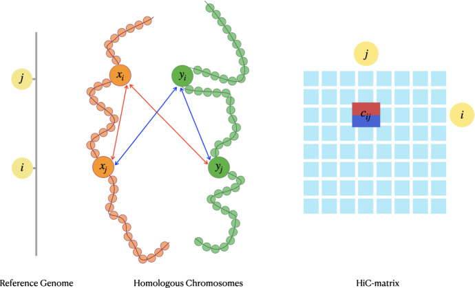
The 3-dimensional (3D) structure of the genome is of significant importance for many cellular processes. In this paper, we study the problem of reconstructing the 3D structure of chromosomes from Hi-C data of diploid organisms, which poses additional challenges compared to the better-studied haploid setting. With the help of techniques from algebraic geometry, we prove that a small amount of phased data is sufficient to ensure finite identifiability, both for noiseless and noisy data. In the light of these results, we propose a new 3D reconstruction method based on semidefinite programming, paired with numerical algebraic geometry and local optimization. The performance of this method is tested on several simulated datasets under different noise levels and with different amounts of phased data. We also apply it to a real dataset from mouse X chromosomes, and we are then able to recover previously known structural features.

Keywords: 3D genome organization; Applied algebraic geometry; Diploid organisms; Hi-C; Numerical algebraic geometry.

Fig. 1

Ambiguity of phased data. Each entry $c_{i,j}$ of the Hi-C matrix corresponds to four different contacts between the two pairs $(x_i,y_i)$ for locus i and $(x_j,y_j)$ for locus j

Fig. 2

Seven different types of contacts between the ith and jth locus

Fig. 3

Examples of reconstructions for varying noise levels, for a chromosome pair with 60 loci, out of which $50\%$ are ambiguous. a–c Show chromosomes simulated with Brownian motion (projected onto the xy-plane), whereas d–e show helix-shaped chromosomes (color figure online)

Fig. 4

Comparison between our reconstruction method, ASHIC and PASTIS. The values are the average over 20 runs, with the error bars showing the standard deviation. All experiments took place with 60 loci, with varying levels of noise, as well as varying numbers of ambiguous loci, uniformly randomly distributed over the chromosomes (color figure online)

Fig. 5

a Reconstruction from a real dataset using our reconstruction method. A dashed line between two beads is used to indicate that there is one or more beads between them, for which we have not given an estimation (due to low contact counts). b Bipartite index for the reconstructed chromosomes. The dashed vertical line indicates the known hinge point at locus 146 (color figure online)

Fig. 6

SNLC reconstructions, without the local optimization step (color figure online)

Fig. 7

a Total contact counts sorted in increasing order. b Ratios between total contact counts. The peak corresponding to the ratio between the 48th and the 47th smallest count is used as a motivation for excluding the 47 loci with smallest total contact from the analysis. c Unambiguity quotients for each of the remaining 296 loci, sorted in increasing order. We consider a locus as ambiguous if this ratio is less than 0.4; otherwise, we consider it as unambiguous (color figure online)

Fig. 8

Logarithmic heat maps for the reassigned contact count matrices obtained from the original Patski dataset and from the SNLC reconstruction: a and b $C^U$; c and d $C^P$; e and f $C^A$. The axis labels correspond to the 500 unambiguous beads, and the 46 ambiguous loci

Fig. 9

Max-norm of the imaginary parts encountered in the numerical algebraic geometry estimation of various loci. Each subfigure corresponds to an ambiguous locus: a–d correspond to the first four loci of the synthetic dataset used in Fig. 3b; e–h correspond to the first four ambiguous loci of the Patski dataset. Each colored line corresponds to a specific choice of 6 unambiguous beads used in the estimation of the locus. Each line connects 40 points, that record the max-norm of the imaginary part of a solution (up to symmetry) found for the corresponding choice of 6 unambiguous beads. The dashed line at 0.15 corresponds to the choice of threshold for when a solution is considered approximately real. Similar figures for the rest of the ambiguous loci in the respective chromosome pairs can be found in the Github repository (color figure online)

References

1. Alfakih AY, Khandani A, Wolkowicz H. Solving euclidean distance matrix completion problems via semidefinite programming. Comput Optim Appl. 1999;12(1):13–30. doi: 10.1023/A:1008655427845. - DOI
1. Belyaeva A, Kubjas K, Sun LJ, Uhler C. Identifying 3D genome organization in diploid organisms via Euclidean distance geometry. SIAM J Math Data Sci. 2022;4(1):204–228. doi: 10.1137/21M1390372. - DOI
1. Breiding P, Rose K, Timme S. Certifying zeros of polynomial systems using interval arithmetic. ACM Trans Math Softw. 2023;49(1):1–14. doi: 10.1145/3580277. - DOI
1. Breiding P, Timme S (2018) HomotopyContinuation.jl: A package for homotopy continuation in Julia. In: Davenport JH, Kauers M, Labahn G, Urban J (eds) Mathematical Software—ICMS 2018. Springer, Cham, pp 458–465
1. Cauer AG, Yardimci G, Vert JP, Varoquaux N, Noble WS (2019) Inferring diploid 3D chromatin structures from Hi-C data. In: 19th International workshop on algorithms in bioinformatics (WABI 2019)
Publication types