What Influence Could the Acceptance of Visitors Cause on the Epidemic Dynamics of a Reinfectious Disease?: A Mathematical Model

Abstract

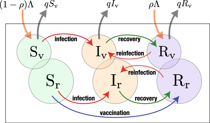
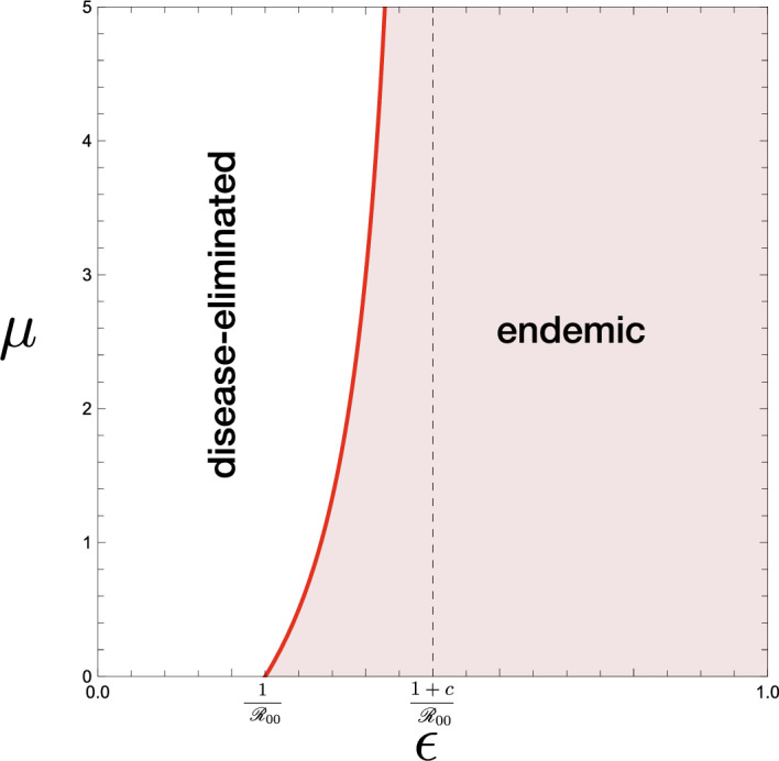
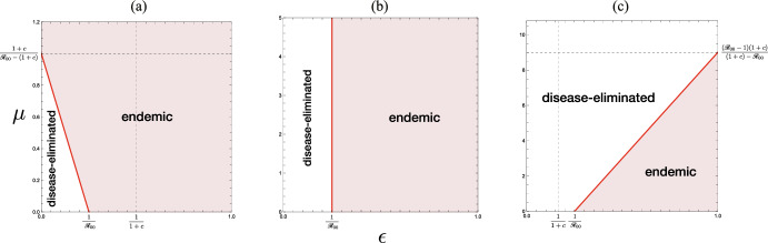
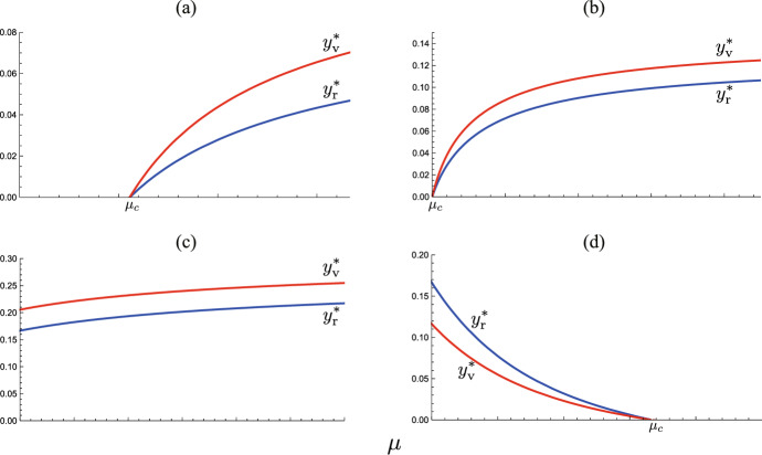
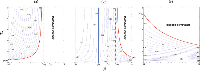
The globalization in business and tourism becomes crucial more and more for the economical sustainability of local communities. In the presence of an epidemic outbreak, there must be such a decision on the policy by the host community as whether to accept visitors or not, the number of acceptable visitors, or the condition for acceptable visitors. Making use of an SIRI type of mathematical model, we consider the influence of visitors on the spread of a reinfectious disease in a community, especially assuming that a certain proportion of accepted visitors are immune. The reinfectivity of disease here means that the immunity gained by either vaccination or recovery is imperfect. With the mathematical results obtained by our analysis on the model for such an epidemic dynamics of resident and visitor populations, we find that the acceptance of visitors could have a significant influence on the disease's endemicity in the community, either suppressive or supportive.

Keywords: Epidemic dynamics; Mathematical model; Ordinary differential equations; Public health; Reinfection.

Fig. 1

Scheme of the model for the epidemic dynamics in a community accepting temporal visitors, given by the system of (1) and (2)

Fig. 2

The dependence of the basic reproduction number ${\mathcal{R}}_0$ given by (4) on parameters $(1-ϵ)\rho$ and $\mu :=m/N$. Numerically drawn with ${\mathcal{R}}_{00}=1.4$

Fig. 3

Temporal variations by the system (5). Numerically drawn with a $(ϵ,\mu ,\rho )=(0.0,0.2,0.1)$ (${\mathcal{R}}_0=7.87$); b $(ϵ,\mu ,\rho )=(0.0,0.5,0.1)$ (${\mathcal{R}}_0=7.73$); c $(ϵ,\mu ,\rho )=(0.1,0.2,0.1)$ (${\mathcal{R}}_0=7.88$); d $(ϵ,\mu ,\rho )=(0.1,0.5,0.8)$ (${\mathcal{R}}_0=6.08$); and commonly ${\mathcal{R}}_{00}=8.0$; $c=1.0$; $\omega =1.0$; $(x_{\text{v}}(0),y_{\text{v}}(0),x_{\text{r}}(0),y_{\text{r}}(0))=(1-\rho ,0.0,0.99,0.01)$. In a, d, the system approaches the disease-eliminated equilibrium, and in b, c, it approaches the endemic equilibrium

Fig. 4

Application of the isocline method for the system with no visitor (8) when a $ϵ{\mathcal{R}}_{00}<1$; b $ϵ{\mathcal{R}}_{00}=1$; (c) $ϵ{\mathcal{R}}_{00}>1$

Fig. 5

Parameter region and boundary indicated by the condition (9). The boundary curve is given by $G(\mu ,\rho )$. a $ϵ<1/(1+c)$; b $ϵ=1/(1+c)$; c $ϵ>1/(1+c)$. Numerically drawn with a $ϵ=0.10$; b $ϵ=0.25$; c $ϵ=0.40$, commonly for $c=3.0$. Solid curves are for $\mu =0.25,0.5,0.75,1.0$ in each figure. Dotted curve indicates $G_{\infty }(\rho )$

Fig. 6

$(ϵ,{\mathcal{R}}_{00})$-dependence of the endemicity, derived from the condition (12) in Theorem 9.1. Numerically drawn for a $\rho =0.0$; b $\rho =0.6$; c $\rho =1.0$, commonly with $c=1.0$. For the region ${\mathrm{\Omega }}_{+}$, the acceptance of visitors may change the endemic situation of the community for the disease-eliminated equilibrium as described in Theorem 9.2, while, for the region ${\mathrm{\Omega }}_{-}$, it may drive the situation of the community approaching the disease-eliminated equilibrium toward the endemic equilibrium as described in Theorem 9.3. For the region out of ${\mathrm{\Omega }}_{-}$ and ${\mathrm{\Omega }}_{+}$, the endemicity is independent of whether the community accepts visitors or not

Fig. 7

Temporal variations of infective subpopulations $y_{\text{r}}$ and $y_{\text{v}}$ by the systems (5) and (8). Numerically drawn for model (8) until $\tau =40$ and model (5) for $\tau >40$, with a $(ϵ,\mu ,\rho )=(0.2,0.9,0.3)$ (${\mathcal{R}}_0=3.55$; $ϵ{\mathcal{R}}_{00}=0.8$); b $(ϵ,\mu ,\rho )=(0.3,0.9,0.3)$ (${\mathcal{R}}_0=3.60$; $ϵ{\mathcal{R}}_{00}=1.2$); c $(ϵ,\mu ,\rho )=(0.3,0.9,0.9)$ (${\mathcal{R}}_0=2.81$; $ϵ{\mathcal{R}}_{00}=1.2$); and commonly ${\mathcal{R}}_{00}=4.0$; $c=1.0$; $\omega =1.0$; $(x_{\text{r}}(0),y_{\text{r}}(0))=(0.99,0.01)$; $(x_{\text{v}}(40),y_{\text{v}}(40))=(1-\rho ,0.0)$. In a and c, the endemicity is changed before and after starting the acceptance of visitors, while in b the system remains at an endemic state before and after it

Fig. 8

$(\rho ,\mu )$-dependence of the endemicity, derived from the condition (9) with the results given by Theorems 8.1, 8.2, and 8.3: a, b $ϵ<1/(1+c)$; c $ϵ>1/(1+c)$. Numerically drawn for a $({\mathcal{R}}_{00},ϵ,c)=(4.0,0.2,1.0)$ ($ϵ{\mathcal{R}}_{00}=0.8$); b $({\mathcal{R}}_{00},ϵ,c)=(4.0,0.3,1.0)$ ($ϵ{\mathcal{R}}_{00}=1.2$); c $({\mathcal{R}}_{00},ϵ,c)=(1.8,0.8,1.0)$ ($ϵ{\mathcal{R}}_{00}=1.44$), each of which satisfies the condition (13) in Corollary 9.1.1

Fig. 9

Parameter region and boundary indicated by the condition (9) with the results given by Theorems 8.1, 8.2, and 8.3 when the community accepts only immune visitors with $\rho =1$. Numerically drawn with ${\mathcal{R}}_{00}=4.0$ and $c=1.0$. Refer to Sect. 9.2

Fig. 10

Parameter region and boundary indicated by the condition the condition (9) with the results given by Theorems 8.1, 8.2, and 8.3 when all visitors accepted by the community is susceptible with $\rho =0$: a ${\mathcal{R}}_{00}>1+c$; b ${\mathcal{R}}_{00}=1+c$; c ${\mathcal{R}}_{00}<1+c$. Numerically drawn with a $c=1.0$; b $c=3.0$; c $c=5.0$, and commonly ${\mathcal{R}}_{00}=4.0$. Refer to Sect. 9.3

Fig. 11

$\mu$-dependence of endemic sizes. Numerically drawn by (10) with a $(ϵ,\rho )=(0.2,0.4)$ ($ϵ{\mathcal{R}}_{00}=0.8$, ${\mu }_c=0.56$); b $(ϵ,\rho )=(0.25,0.4)$ ($ϵ{\mathcal{R}}_{00}=1.0$, ${\mu }_c=0.0$, ${\rho }_c=0.67$), c $(ϵ,\rho )=(0.3,0.1)$ ($ϵ{\mathcal{R}}_{00}=1.2$, ${\mu }_c<0$, ${\rho }_c=0.40$), d $(ϵ,\rho )=(0.3,0.8)$ ($ϵ{\mathcal{R}}_{00}=1.2$, ${\mu }_c=1.67$, ${\rho }_c=0.40$), and commonly ${\mathcal{R}}_{00}=4.0$; $c=1.0$

Fig. 12

$(\rho ,\mu )$-dependence of the endemic size $y_{\text{r}}^{\ast }$. Numerically drawn contour maps for three cases correspond to those in Fig. 8: a $ϵ{\mathcal{R}}_{00}=0.8$; b $ϵ{\mathcal{R}}_{00}=1.2$ and ${\rho }_c=0.40$; c $ϵ{\mathcal{R}}_{00}=1.44$ and ${\rho }_c=-3.31$, where the parameter values are respectively the same as in Fig. 8

Fig. 13

Classification of the parameter region of $(ϵ,\rho )$ according to the $\mu$-dependence of the change in the endemic size. Numerically drawn with ${\mathcal{R}}_{00}=4.0$ and $c=1.0$. Regions ${\mathrm{\Omega }}_{\pm }$ correspond to those in Fig. 6

Fig. 14

Application of the isocline method for the system (B1) when the condition (7) is (a) not satisfied; (b) satisfied

References

1. Agusto FB. Mathematical model of Ebola transmission dynamics with relapse and reinfection. Math Biosci. 2017;283:48–59. doi: 10.1016/j.mbs.2016.11.002. - DOI - PubMed
1. Arias CF, Acosta FJ, Fernandez-Arias C. Killing the competition: a theoretical framework for liver-stage malaria. Open Biol. 2022;12:210341. doi: 10.1098/rsob.210341. - DOI - PMC - PubMed
1. Athayde GM, Alencar AP. Forecasting Covid-19 in the United Kingdom: a dynamic SIRD model. PlOS one. 2022;17(8):e0271577. doi: 10.1371/journal.pone.0271577. - DOI - PMC - PubMed
1. Bavel JJ, Baicker K, Boggio PS, Capraro V, Cichocka A, Cikara M, Crockett MJ, Crum AJ, Douglas KM, Druckman JN, Drury J. Using social and behavioural science to support COVID-19 pandemic response. Nat Hum Behav. 2020;4(5):460–471. doi: 10.1038/s41562-020-0884-z. - DOI - PubMed
1. Brauer F. Mathematical epidemiology: past, present, and future. Infect Dis Model. 2017;2:113–127. doi: 10.1016/j.idm.2017.02.001. - DOI - PMC - PubMed
LinkOut - more resources