Pseudo-value regression trees

Abstract

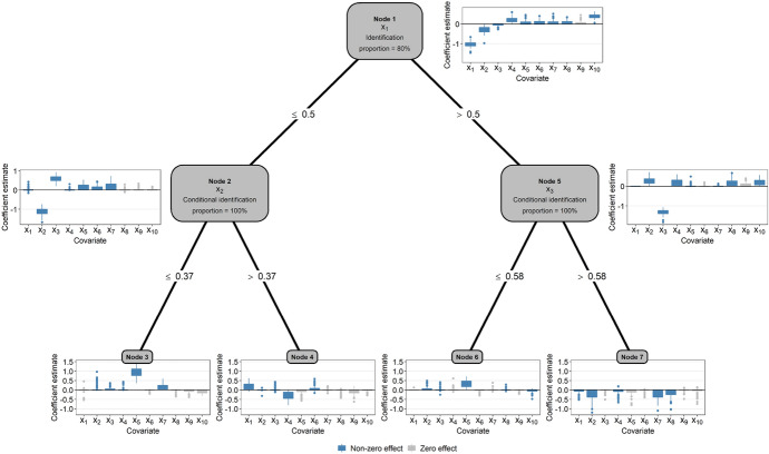
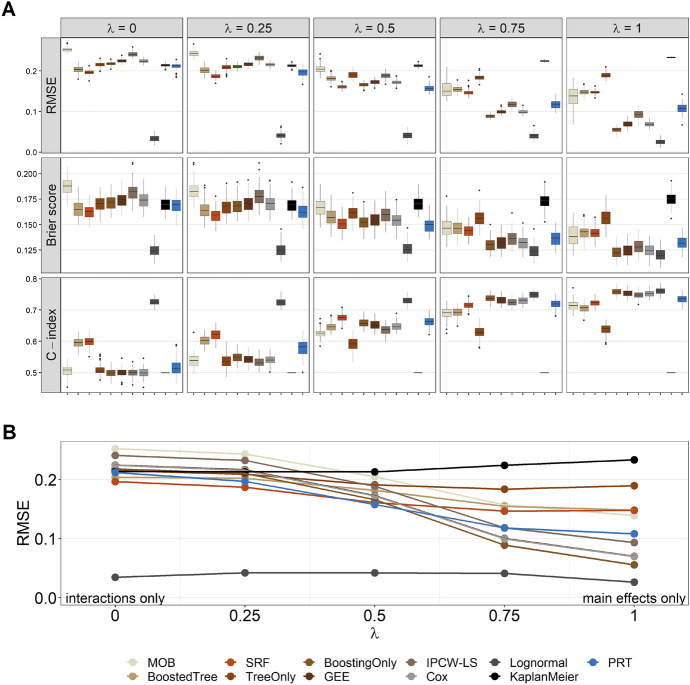
This paper presents a semi-parametric modeling technique for estimating the survival function from a set of right-censored time-to-event data. Our method, named pseudo-value regression trees (PRT), is based on the pseudo-value regression framework, modeling individual-specific survival probabilities by computing pseudo-values and relating them to a set of covariates. The standard approach to pseudo-value regression is to fit a main-effects model using generalized estimating equations (GEE). PRT extend this approach by building a multivariate regression tree with pseudo-value outcome and by successively fitting a set of regularized additive models to the data in the nodes of the tree. Due to the combination of tree learning and additive modeling, PRT are able to perform variable selection and to identify relevant interactions between the covariates, thereby addressing several limitations of the standard GEE approach. In addition, PRT include time-dependent effects in the node-wise models. Interpretability of the PRT fits is ensured by controlling the tree depth. Based on the results of two simulation studies, we investigate the properties of the PRT method and compare it to several alternative modeling techniques. Furthermore, we illustrate PRT by analyzing survival in 3,652 patients enrolled for a randomized study on primary invasive breast cancer.

Keywords: Gradient boosting; Interactions; Model trees; Pseudo-values; Survival probabilities.

Fig. 1

A Illustration of pseudo-values obtained from two data sets with $n=1000$ individuals each ($0\le t_k\le 6$, adapted from Andersen and Pohar 2010). Panel (a) refers to an individual with ${\tilde{T}}_i=T_i=2$ in a censoring-free data set, whereas the other panels refer to a censored individual with ${\tilde{T}}_i=2,{\mathrm{\Delta }}_i=0$ (Panel (b)) and an uncensored individual with ${\tilde{T}}_i=2,{\mathrm{\Delta }}_i=1$ (Panel (c)) in a data set with $50\%$ right-censored survival times. In the censoring-free scenario (a), the pseudo-value at time $t_k$ is simply a binary function indicating whether the individual is still event-free at $t_k$ (${\widehat{\theta }}_i(t_k)=1$) or not (${\widehat{\theta }}_i(t_k)=0$). In the scenario with $50\%$ censoring, the individuals in (b) and (c) have exactly the same pseudo-values up to their common observed survival time (${\tilde{T}}_i=2$), showing a monotonically increasing pattern. After ${\tilde{T}}_i=2$, the pseudo-values of the two individuals differ: While the censoring of the individual in (b) caused ${\widehat{\theta }}_i(t_k)$ to become monotonically decreasing after ${\tilde{T}}_i=2$, the observed event in (c) caused ${\widehat{\theta }}_i(t_k)$ to drop to a negative value at ${\tilde{T}}_i=2$ and to increase afterwards. B Histograms of pseudo-values at different time points in the data set with $50\%$ right-censored survival times from (A). The colors indicate the status of the individuals at the respective time points (dead, censored, still at risk). Pseudo-values of individuals that were observed to experience the event of interest before $t_k$ are negative, whereas pseudo-values are $\ge 1$ in individuals that are still at risk at $t_k$. Obviously, the distribution of the pseudo-values is strongly dependent on both the censoring pattern and the time point of interest

Fig. 2

Schematic overview of the PRT method

Fig. 3

The plot illustrates the data-generating process of the first simulation study. The boxplots below the terminal nodes were generated from a random sample of size $n=1000$. They present the distributions of the survival times on the log scale

Fig. 4

Results of the first simulation study. The boxplots present the RMSE, bias, Brier score, and C-index values that were obtained by applying the PRT method with varying tree depths ($D\in \{0,1,2,3,4,5\}$) to the training data and by evaluating the resulting model fits on the test data. Note that $D=2$ corresponds to the true tree depth, as defined by the data-generating process

Fig. 5

Results of the first simulation study ($D=2$, 100 Monte Carlo replications). The plot presents the percentages of correctly identified split variables as well as boxplots of the coefficient estimates obtained from the node-wise boosting fits. In Nodes 2–7, the percentages and coefficient estimates are conditional on having identified the split variable in the parent node. Blue and gray boxplots refer to informative covariates (defined by a non-zero effect in the present or in any of the lower-level nodes) and non-informative covariates, respectively. Coefficient estimates are zero if the respective base-learners were not selected by the gradient boosting algorithm

Fig. 6

Results of the second simulation study ($D=2$, 100 Monte Carlo replications). A Boxplots of the RMSE, Brier score and C-index values, as obtained by evaluating the model fits on the 100 test data sets. B Mean RMSE values (across the replications). Note that MOB did not converge in some of the replications (failure rates = $2\%,1\%,2\%,0\%$, and $1\%$ for $\lambda =0,0.25,0.5,0.75$, and $1$, respectively). The results of these models were excluded from the plots

Fig. 7

Analysis of disease-free survival in the SUCCESS-A study data. The figure presents the results obtained from fitting a PRT model with $D=3$, showing the selected split variables and the sizes of the patient subgroups in the nodes. The blue bars refer to the base-learners selected in the node-wise boosting models. The blue dots and the black lines refer to the fitted values and their averages in the terminal nodes. In Node 4, the mean estimated DFS function of the group of “triple negative” patients (i.e. negative ER, PR and HER2, von Minckwitz et al. 2012) is marked red. The green line refers to mean estimated DFS in the group of HER2 receptor-positive patients. The colored lines in Node 9 refer to the mean estimated DFS functions stratified by tumor stage (light red = pT1, dark red = pT4)

References

1. Andersen PK, Pohar Perme M (2010) Pseudo-observations in survival analysis. Statist Methods Med Res 19:71–9910.1177/0962280209105020 - DOI - PubMed
1. Andersen PK, Klein JP, Rosthøj S (2003) Generalised linear models for correlated pseudo-observations, with applications to multi-state models. Biometrika 90:15–2710.1093/biomet/90.1.15 - DOI
1. Bacchetti P, Segal MR (1995) Survival trees with time-dependent covariates: Application to estimating changes in the incubation period of AIDS. Lifetime Data Anal 1:35–47 10.1007/BF00985256 - DOI - PubMed
1. Binder N, Gerds TA, Andersen PK (2014) Pseudo-observations for competing risks with covariate dependent censoring. Lifetime Data Anal 20:303–315 10.1007/s10985-013-9247-7 - DOI - PMC - PubMed
1. Breiman L, Friedman J, Stone CJ, Olshen RA (1984) Classification and regression trees. Taylor & Francis, New York
LinkOut - more resources