Statistics of maximum photon penetration depth in a two-layer diffusive medium

Abstract

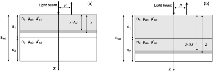
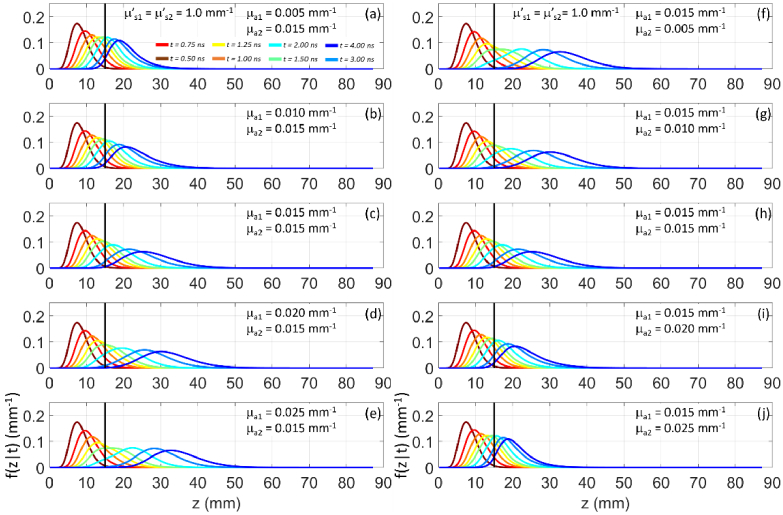
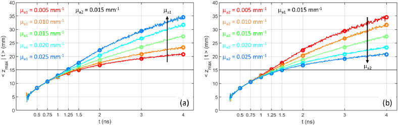
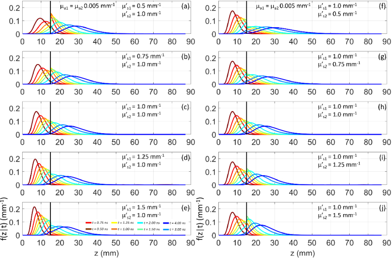
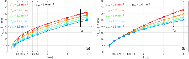
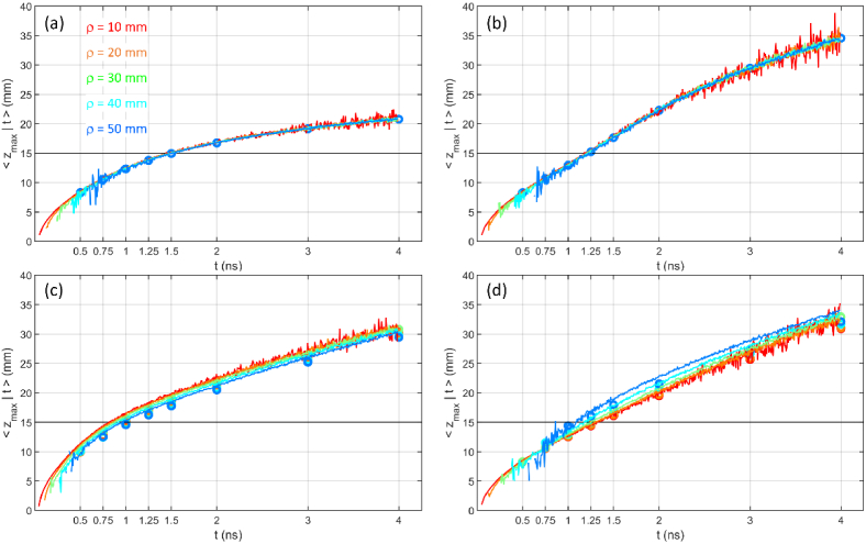
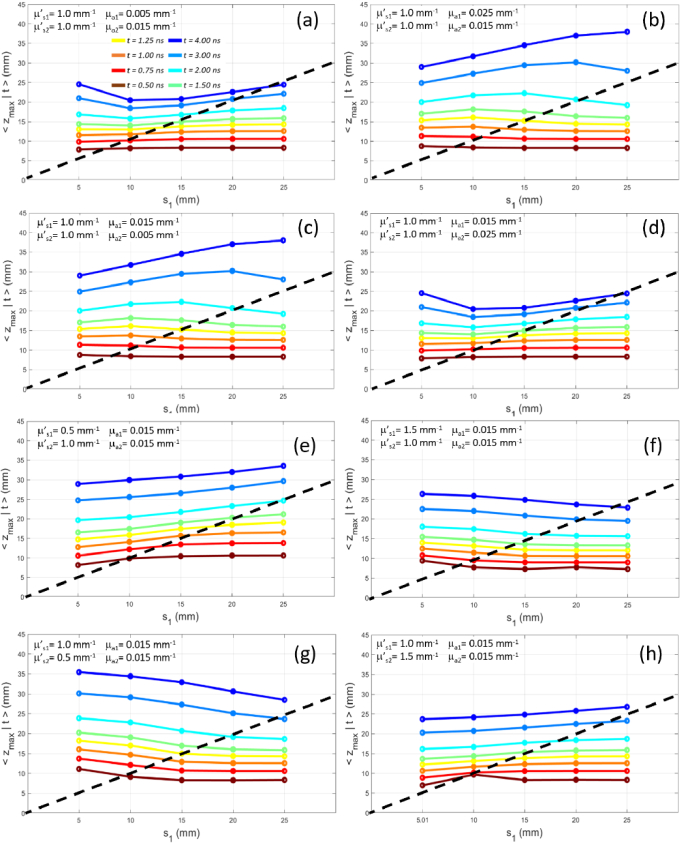
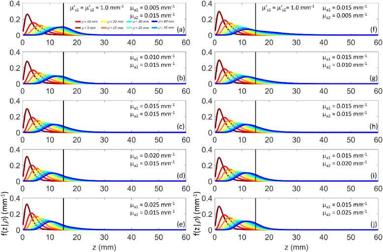
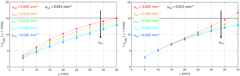
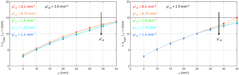
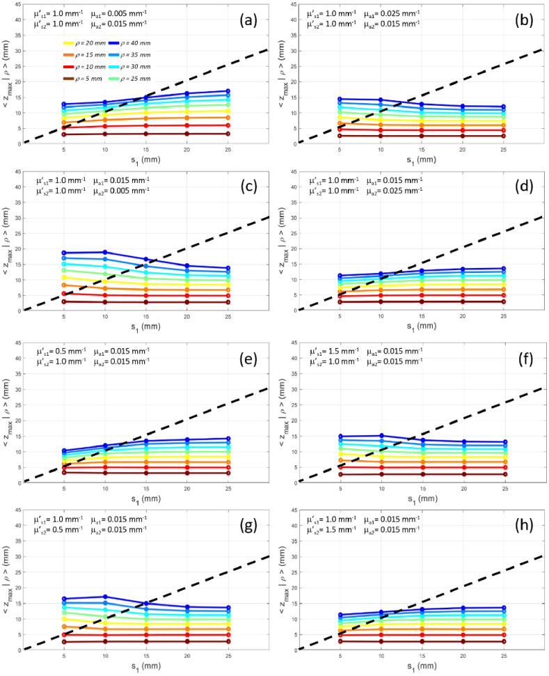
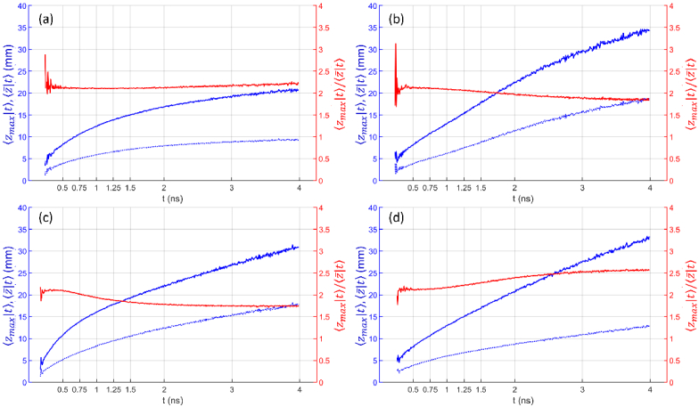
We present numerical results for the probability density function f(z) and for the mean value of photon maximum penetration depth ‹z_max› in a two-layer diffusive medium. Both time domain and continuous wave regime are considered with several combinations of the optical properties (absorption coefficient, reduced scattering coefficient) of the two layers, and with different geometrical configurations (source detector distance, thickness of the upper layer). Practical considerations on the design of time domain and continuous wave systems are derived. The methods and the results are of interest for many research fields such as biomedical optics and advanced microscopy.

Fig. 1.

Scheme for the implementation of the numerical method. (a) if $z<s_1$ the model for reflectance from a homogeneous slab of thickness z is used; (b) if $z>s_1$ the model for reflectance from a two-layer slab with $s_2=z$ is used.

Fig. 2.

$f(z|t)$ as a function of z for $t=0.50,0.75,1.00,1.25,1.5,2.0,3.0,4.0\text{ns}$ (color code from brown to blue) for a two-layer medium ( $s_1=15\text{mm}$ , $s_2=75\text{mm}$ , $n_1=n_2=1.4$ , ${\mu }_{s1}^{\mathrm{\prime }}={\mu }_{s2}^{\mathrm{\prime }}=1.0\text{m}{\text{m}}^{-1}$ ). (a)-(e): variable ${\mu }_{a1}=0.005,0.010,0.015,0.020,0.025\text{m}{\text{m}}^{-1}$ , fixed ${\mu }_{a2}=0.015\text{m}{\text{m}}^{-1}$ ; (f)-(j): fixed ${\mu }_{a1}=0.015\text{m}{\text{m}}^{-1}$ , variable ${\mu }_{a2}=0.005,0.010,0.015,0.020,0.025\text{m}{\text{m}}^{-1}$ . In all cases $\rho =30\text{mm}$ , $n_{e1}=n_{e2}=1.0$ .

Fig. 3.

$⟨z_{max}|t⟩$ as a function of t for a two-layer medium ( $s_1=15\text{mm}$ , $s_2=75\text{mm}$ , $n_1=n_2=1.4$ , ${\mu }_{s1}^{\mathrm{\prime }}={\mu }_{s2}^{\mathrm{\prime }}=1.0\text{m}{\text{m}}^{-1}$ ). (a) variable ${\mu }_{a1}=0.005,0.010,0.015,0.020,0.025\text{m}{\text{m}}^{-1}$ , fixed ${\mu }_{a2}=0.015\text{m}{\text{m}}^{-1}$ ; (b) fixed ${\mu }_{a1}=0.015\text{m}{\text{m}}^{-1}$ , variable ${\mu }_{a2}=0.005,0.010,0.015,0.020,0.025\text{m}{\text{m}}^{-1}$ . In all cases $\rho =30\text{mm}$ , $n_{e1}=n_{e2}=1.0$ . Circles are DE results, lines are MC results.

Fig. 4.

$f(z|t)$ as a function of z for $t=0.50,0.75,1.00,1.25,1.5,2.0,3.0,4.0\text{ns}$ (color code from brown to blue) for a two-layer medium ( $s_1=15\text{mm}$ , $s_2=75\text{mm}$ , $n_1=n_2=1.4$ , ${\mu }_{a1}={\mu }_{a2}=0.015\text{m}{\text{m}}^{-1}$ ). (a)-(e): variable ${\mu }_{s1}^{\mathrm{\prime }}=0.5,0.75,1.0,1.25,1.5\text{m}{\text{m}}^{-1}$ , fixed ${\mu }_{s2}^{\mathrm{\prime }}=1.0\text{m}{\text{m}}^{-1}$ ; (f)-(j): fixed ${\mu }_{s1}^{\mathrm{\prime }}=1.0\text{m}{\text{m}}^{-1}$ , variable ${\mu }_{s2}^{\mathrm{\prime }}=0.5,0.75,1.0,1.25,1.5\text{m}{\text{m}}^{-1}$ . In all cases $\rho =30mm$ , $n_{e1}=n_{e2}=1.0$ .

Fig. 5.

$⟨z_{max}|t⟩$ as a function of t for a two-layer medium ( $s_1=15\text{mm}$ , $s_2=75\text{mm}$ , $n_1=n_2=1.4$ , ${\mu }_{a1}={\mu }_{a2}=0.015\text{m}{\text{m}}^{-1}$ ). (a) variable ${\mu }_{s1}^{\mathrm{\prime }}=0.5,0.75,1.0,1.25,1.5\text{m}{\text{m}}^{-1}$ , fixed ${\mu }_{s2}^{\mathrm{\prime }}=1.0\text{m}{\text{m}}^{-1}$ ; (b) fixed ${\mu }_{s1}^{\mathrm{\prime }}=1.0\text{m}{\text{m}}^{-1}$ , variable ${\mu }_{s2}^{\mathrm{\prime }}=0.5,0.75,1.0,1.25,1.5\text{m}{\text{m}}^{-1}$ . In all cases $\rho =30\text{mm}$ , $n_{e1}=n_{e2}=1.0$ . Circles are DE results, lines are MC results.

Fig. 6.

$⟨z_{max}|t⟩$ as a function of t for a two-layer medium ( $s_1=15\text{mm}$ , $s_2=75\text{mm}$ , $n_1=n_2=1.4$ ). for different values of $\rho =10,20,30,40,50\text{mm}$ . (a) different absorption ( ${\mu }_{a1}=0.005\text{m}{\text{m}}^{-1}$ , ${\mu }_{a2}=0.015\text{m}{\text{m}}^{-1}$ ), same scattering ( ${\mu }_{s1}^{\mathrm{\prime }}={\mu }_{s2}^{\mathrm{\prime }}=1.0\text{m}{\text{m}}^{-1}$ ); (b) different absorption ( ${\mu }_{a1}=0.015\text{m}{\text{m}}^{-1}$ , ${\mu }_{a2}=0.005\text{m}{\text{m}}^{-1}$ ), same scattering ( ${\mu }_{s1}^{\mathrm{\prime }}={\mu }_{s2}^{\mathrm{\prime }}=1.0\text{m}{\text{m}}^{-1}$ ); (c) same absorption ( ${\mu }_{a1}={\mu }_{a2}=0.015\text{m}{\text{m}}^{-1}$ ), different scattering ( ${\mu }_{s1}^{\mathrm{\prime }}=0.5\text{m}{\text{m}}^{-1}$ , ${\mu }_{s2}^{\mathrm{\prime }}=1.0\text{m}{\text{m}}^{-1}$ ); (d) same absorption ( ${\mu }_{a1}={\mu }_{a2}=0.015\text{m}{\text{m}}^{-1}$ ), different scattering ( ${\mu }_{s1}^{\mathrm{\prime }}=1.0\text{m}{\text{m}}^{-1}$ , ${\mu }_{s2}^{\mathrm{\prime }}=0.5\text{m}{\text{m}}^{-1}$ ). In all cases $n_{e1}=n_{e2}=1.0$ . Circles are DE results, lines are MC results.

Fig. 7.

$⟨z_{max}|t⟩$ at different time of flight $t=0.50,0.75,1.00,1.25,1.5,2.0,3.0,4.0\text{ns}$ (color code from brown to blue) as a function of the thickness of the upper layer $s_1=5,10,15,20,25\text{mm}$ for a two-layer medium with constant total thickness ( $s_{\mathit{\text{tot}}}=90\text{mm}$ , $n_1=n_2=1.4$ ). Panels (a)-(d) have same scattering ( ${\mu }_{s1}^{\mathrm{\prime }}={\mu }_{s2}^{\mathrm{\prime }}=1.0\text{m}{\text{m}}^{-1}$ ) and different absorption: (a) ${\mu }_{a1}=0.005\text{m}{\text{m}}^{-1}$ , ${\mu }_{a2}=0.015\text{m}{\text{m}}^{-1}$ ; (b) ${\mu }_{a1}=0.025\text{m}{\text{m}}^{-1}$ , ${\mu }_{a2}=0.015\text{m}{\text{m}}^{-1}$ ; (c) ${\mu }_{a1}=0.015\text{m}{\text{m}}^{-1}$ , ${\mu }_{a2}=0.005\text{m}{\text{m}}^{-1}$ ; (d) ${\mu }_{a1}=0.015\text{m}{\text{m}}^{-1}$ , ${\mu }_{a2}=0.025\text{m}{\text{m}}^{-1}$ . Panels (e)-(h) have same absorption ( ${\mu }_{a1}={\mu }_{a2}=0.015\text{m}{\text{m}}^{-1}$ ) and different scattering: (e) ${\mu }_{s1}^{\mathrm{\prime }}=0.5\text{m}{\text{m}}^{-1}$ , ${\mu }_{s2}^{\mathrm{\prime }}=1.0\text{m}{\text{m}}^{-1}$ ); (f) ${\mu }_{s1}^{\mathrm{\prime }}=1.5\text{m}{\text{m}}^{-1}$ , ${\mu }_{s2}^{\mathrm{\prime }}=1.0\text{m}{\text{m}}^{-1}$ ); (g) ${\mu }_{s1}^{\mathrm{\prime }}=1.0\text{m}{\text{m}}^{-1}$ , ${\mu }_{s2}^{\mathrm{\prime }}=0.5\text{m}{\text{m}}^{-1}$ ); (h) ${\mu }_{s1}^{\mathrm{\prime }}=1.0\text{m}{\text{m}}^{-1}$ , ${\mu }_{s2}^{\mathrm{\prime }}=1.5\text{m}{\text{m}}^{-1}$ ). In all cases we set $\rho =30\text{mm}$ , $n_{e1}=n_{e2}=1.0$ . The dashed line is the unity line for which $⟨z_{max}|t⟩=s_1$ .

Fig. 8.

$f(z|\rho )$ as a function of z for $\rho =5,10,15,20,25,30,35,40\text{mm}$ (color code from brown to blue) for a two-layer medium ( $s_1=15\text{mm}$ , $s_2=75\text{mm}$ , $n_1=n_2=1.4$ , ${\mu }_{s1}^{\mathrm{\prime }}={\mu }_{s2}^{\mathrm{\prime }}=1.0\text{mm}$ ). (a)-(e) variable ${\mu }_{a1}=0.005,0.010,0.015,0.020,0.025\text{m}{\text{m}}^{-1}$ , fixed ${\mu }_{a2}=0.015\text{m}{\text{m}}^{-1}$ ; (f)-(j) fixed ${\mu }_{a1}=0.015\text{m}{\text{m}}^{-1}$ , variable ${\mu }_{a2}=0.005,0.010,0.015,0.020,0.025\text{m}{\text{m}}^{-1}$ .

Fig. 9.

$⟨z_{max}|\rho ⟩$ as a function of $\rho$ for a two-layer medium ( $s_1=15\text{mm}$ , $s_2=75\text{mm}$ , $n_1=n_2=1.4$ , ${\mu }_{s1}^{\mathrm{\prime }}={\mu }_{s2}^{\mathrm{\prime }}=1.0\text{m}{\text{m}}^{-1}$ ). (a) variable ${\mu }_{a1}=0.005,0.010,0.015,0.020,0.025\text{m}{\text{m}}^{-1}$ , fixed ${\mu }_{a2}=0.015\text{m}{\text{m}}^{-1}$ ; (b) fixed ${\mu }_{a1}=0.015\text{m}{\text{m}}^{-1}$ , variable ${\mu }_{a2}=0.005,0.010,0.015,0.020,0.025\text{m}{\text{m}}^{-1}$ . Circles are DE results, crosses are MC results. Lines connect MC results to guide the eye.

Fig. 10.

$f(z|\rho )$ as a function of z for $\rho =5,10,15,20,25,30,35,40\text{mm}$ (color code from brown to blue) for a two-layer medium ( $s_1=15\text{mm}$ , $s_2=75\text{mm}$ , $n_1=n_2=1.4$ , ${\mu }_{a1}={\mu }_{a2}=0.015\text{m}{\text{m}}^{-1}$ ). (a)-(e) variable ${\mu }_{s1}^{\mathrm{\prime }}=0.5,0.75,1.0,1.25,1.5\text{m}{\text{m}}^{-1}$ , from top to bottom) and fixed ${\mu }_{s2}^{\mathrm{\prime }}=1.0\text{m}{\text{m}}^{-1}$ ; (f)-(j) fixed ${\mu }_{s1}^{\mathrm{\prime }}=1.0\text{m}{\text{m}}^{-1}$ and variable ${\mu }_{s2}^{\mathrm{\prime }}=0.5,0.75,1.0,\text{m}{\text{m}}^{-1}$ , from top to bottom).

Fig. 11.

$⟨z_{max}|\rho ⟩$ as a function of $\rho$ for a two-layer medium ( $s_1=15\text{mm}$ , $s_2=75\text{mm}$ , $n_1=n_2=1.4$ , ${\mu }_{a1}={\mu }_{a2}=0.015\text{m}{\text{m}}^{-1}$ ). (a) variable ${\mu }_{s1}^{\mathrm{\prime }}=0.5,0.75,1.0,1.25,1.5\text{m}{\text{m}}^{-1}$ and fixed ${\mu }_{s2}^{\mathrm{\prime }}=1.0\text{m}{\text{m}}^{-1}$ ; (b) fixed ${\mu }_{s1}^{\mathrm{\prime }}=1.0\text{m}{\text{m}}^{-1}$ and variable ${\mu }_{s2}^{\mathrm{\prime }}=0.5,0.75,1.0,1.25,1.5\text{m}{\text{m}}^{-1}$ . Circles are DE results, crosses are MC results, lines connect MC results to guide the eye.

Fig. 12.

$⟨z_{max}|\rho ⟩$ for $\rho =5,10,15,20,25,30,35,40\text{mm}$ (color code from brown to blue) as a function of the thickness of the upper layer $s_1=5,10,15,20,25\text{mm}$ for a two-layer medium with constant total thickness ( $s_{\mathit{\text{tot}}}=90\text{mm}$ , $n_1=n_2=1.4$ ). Panels (a)-(d) have same scattering ( ${\mu }_{s1}^{\mathrm{\prime }}={\mu }_{s2}^{\mathrm{\prime }}=1.0\text{m}{\text{m}}^{-1}$ ) and different absorption: (a) ${\mu }_{a1}=0.005\text{m}{\text{m}}^{-1}$ , ${\mu }_{a2}=0.015\text{m}{\text{m}}^{-1}$ ; (b) ${\mu }_{a1}=0.025\text{m}{\text{m}}^{-1}$ , ${\mu }_{a2}=0.015\text{m}{\text{m}}^{-1}$ ; (c) ${\mu }_{a1}=0.015\text{m}{\text{m}}^{-1}$ , ${\mu }_{a2}=0.005\text{m}{\text{m}}^{-1}$ ; (d) ${\mu }_{a1}=0.015\text{m}{\text{m}}^{-1}$ , ${\mu }_{a2}=0.025\text{m}{\text{m}}^{-1}$ . Panels (e)-(h) have same absorption ( ${\mu }_{a1}={\mu }_{a2}=0.015\text{m}{\text{m}}^{-1}$ ) and different scattering: (e) ${\mu }_{s1}^{\mathrm{\prime }}=0.5\text{m}{\text{m}}^{-1}$ , ${\mu }_{s2}^{\mathrm{\prime }}=1.0\text{m}{\text{m}}^{-1}$ ); (f) ${\mu }_{s1}^{\mathrm{\prime }}=1.5\text{m}{\text{m}}^{-1}$ , ${\mu }_{s2}^{\mathrm{\prime }}=1.0\text{m}{\text{m}}^{-1}$ ); (g) ${\mu }_{s1}^{\mathrm{\prime }}=1.0\text{m}{\text{m}}^{-1}$ , ${\mu }_{s2}^{\mathrm{\prime }}=0.5\text{m}{\text{m}}^{-1}$ ); (h) ${\mu }_{s1}^{\mathrm{\prime }}=1.0\text{m}{\text{m}}^{-1}$ , ${\mu }_{s2}^{\mathrm{\prime }}=1.5\text{m}{\text{m}}^{-1}$ ). The dashed line is the unity line for which $⟨z_{max}|\rho ⟩=s_1$ .

Fig. 13.

$⟨z_{max}|t⟩$ (blue solid line), $⟨\overline{z}|t⟩$ (blue dashed line) and ratio $⟨z_{max}\mid t⟩/⟨\overline{z}\mid t⟩$ (red line) as a function of t for a two-layer medium ( $s_1=15\text{mm}$ , $s_2=75\text{mm}$ , $n_1=n_2=1.4$ ) for $\rho =30\text{mm}$ . (a) different absorption ( ${\mu }_{a1}=0.005\text{m}{\text{m}}^{-1}$ , ${\mu }_{a2}=0.015\text{m}{\text{m}}^{-1}$ ), same scattering ( ${\mu }_{s1}^{\mathrm{\prime }}={\mu }_{s2}^{\mathrm{\prime }}=1.0\text{m}{\text{m}}^{-1}$ ); (b) different absorption ( ${\mu }_{a1}=0.015\text{m}{\text{m}}^{-1}$ , ${\mu }_{a2}=0.005\text{m}{\text{m}}^{-1}$ ), same scattering ( ${\mu }_{s1}^{\mathrm{\prime }}={\mu }_{s2}^{\mathrm{\prime }}=1.0\text{m}{\text{m}}^{-1}$ ); (c) same absorption ( ${\mu }_{a1}={\mu }_{a2}=0.015\text{m}{\text{m}}^{-1}$ ), different scattering ( ${\mu }_{s1}^{\mathrm{\prime }}=0.5\text{m}{\text{m}}^{-1}$ , ${\mu }_{s2}^{\mathrm{\prime }}=1.0\text{m}{\text{m}}^{-1}$ ); (d) same absorption ( ${\mu }_{a1}={\mu }_{a2}=0.015\text{m}{\text{m}}^{-1}$ ), different scattering ( ${\mu }_{s1}^{\mathrm{\prime }}=1.0\text{m}{\text{m}}^{-1}$ , ${\mu }_{s2}^{\mathrm{\prime }}=0.5\text{m}{\text{m}}^{-1}$ ). In all cases $n_{e1}=n_{e2}=1.0$ .

Fig. 14.

$⟨z_{max}\mid t⟩$ (blue solid line), $⟨\overline{z}\mid t⟩$ (blue dashed line), and ratio $⟨z_{max}\mid t⟩/⟨\overline{z}\mid t⟩$ (red line) as a function of ρ for a two-layer medium ( $s_1=15\text{mm}$ , $s_2=75\text{mm}$ , $n_1=n_2=1.4$ ). (a) different absorption ( ${\mu }_{a1}=0.005\text{m}{\text{m}}^{-1}$ , ${\mu }_{a2}=0.015\text{m}{\text{m}}^{-1}$ ), same scattering ( ${\mu }_{s1}^{\mathrm{\prime }}={\mu }_{s2}^{\mathrm{\prime }}=1.0\text{m}{\text{m}}^{-1}$ ); (b) different absorption ( ${\mu }_{a1}=0.015\text{m}{\text{m}}^{-1}$ , ${\mu }_{a2}=0.005\text{m}{\text{m}}^{-1}$ ), same scattering ( ${\mu }_{s1}^{\mathrm{\prime }}={\mu }_{s2}^{\mathrm{\prime }}=1.0\text{m}{\text{m}}^{-1}$ ); (c) same absorption ( ${\mu }_{a1}={\mu }_{a2}=0.015\text{m}{\text{m}}^{-1}$ ), different scattering ( ${\mu }_{s1}^{\mathrm{\prime }}=0.5\text{m}{\text{m}}^{-1}$ , ${\mu }_{s2}^{\mathrm{\prime }}=1.0\text{m}{\text{m}}^{-1}$ ); (d) same absorption ( ${\mu }_{a1}={\mu }_{a2}=0.015\text{m}{\text{m}}^{-1}$ ), different scattering ( ${\mu }_{s1}^{\mathrm{\prime }}=1.0\text{m}{\text{m}}^{-1}$ , ${\mu }_{s2}^{\mathrm{\prime }}=0.5\text{m}{\text{m}}^{-1}$ ). In all cases $n_{e1}=n_{e2}=1.0$ .

References

1. Ayaz H., Baker W. B., Blaney G., et al. , “Optical imaging and spectroscopy for the study of the human brain: status report,” Neurophotonics 9(S2), S24001001 (2022).10.1117/1.NPh.9.S2.S24001 - DOI - PMC - PubMed
1. Grassi B., Quaresima V., “Near-infrared spectroscopy and skeletal muscle oxidative function in vivo in health and disease: a review from an exercise physiology perspective,” J. Biomed. Opt. 21(9), 091313 (2016).10.1117/1.JBO.21.9.091313 - DOI - PubMed
1. Cortese L., Presti G. L., Zanoletti M., et al. , “The LUCA device: a multi-modal platform combining diffuse optics and ultrasound imaging for thyroid cancer screening,” Biomed. Opt. Express 12(6), 3392–3409 (2021).10.1364/BOE.416561 - DOI - PMC - PubMed
1. Pandiselvam R., Prithviraj V., Manikantan M. R., et al. , “Recent advancements in NIR spectroscopy for assessing the quality and safety of horticultural products: A comprehensive review,” Front. Nutr. 9, 973457 (2022).10.3389/fnut.2022.973457 - DOI - PMC - PubMed
1. Schimleck L., Ma T., Inagaki T., et al. , “Review of near infrared hyperspectral imaging applications related to wood and wood products,” Appl. Spectrosc. Rev. 58(9), 585–609 (2023).10.1080/05704928.2022.2098759 - DOI
LinkOut - more resources