Building Fluorescence Lifetime Maps Photon-by-Photon by Leveraging Spatial Correlations

Abstract

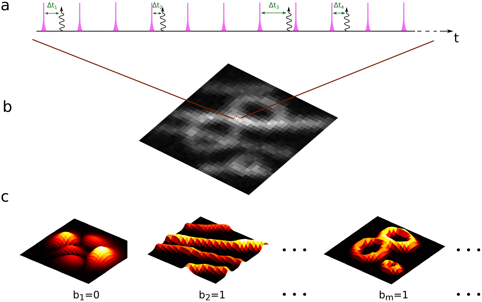
Fluorescence lifetime imaging microscopy (FLIM) has become a standard tool in the quantitative characterization of subcellular environments. However, quantitative FLIM analyses face several challenges. First, spatial correlations between pixels are often ignored as signal from individual pixels is analyzed independently thereby limiting spatial resolution. Second, existing methods deduce photon ratios instead of absolute lifetime maps. Next, the number of fluorophore species contributing to the signal is unknown, while excited state lifetimes with <1 ns difference are difficult to discriminate. Finally, existing analyses require high photon budgets and often cannot rigorously propagate experimental uncertainty into values over lifetime maps and number of species involved. To overcome all of these challenges simultaneously and self-consistently at once, we propose the first doubly nonparametric framework. That is, we learn the number of species (using Beta-Bernoulli process priors) and absolute maps of these fluorophore species (using Gaussian process priors) by leveraging information from pulses not leading to observed photon. We benchmark our framework using a broad range of synthetic and experimental data and demonstrate its robustness across a number of scenarios including cases where we recover lifetime differences between species as small as 0.3 ns with merely 1000 photons.

Keywords: Bayesian; Beta-Bernoulli; FLIM; Gaussian process; confocal; lifetime imaging.

Figure 1.

Cartoon illustration of a typical FLIM experiment and the BNP-FLIM framework. (a) Every spot in the specimen is illuminated by a train of laser pulses, designated by pink spikes, where a fraction of them lead to the detection of photons, shown by curly arrows. The photon arrival times, $\Delta t_k$, are recorded and used in FLIM analysis to infer the number of fluorophore species as well as their associated spatial maps and corresponding lifetimes. (b) The sets of photons drawn from all spots are arranged into a two-dimensional pixel array representing the raw FLIM data. (c) The Bayesian nonparametric FLIM (BNP-FLIM) framework models the input data (nominally) assuming an infinite number of species. To each species are associated a nominally infinite number of candidate spatial maps for how the fluorophores are distributed. Eventually, as shown in (c), our method determines: (1) which species are warranted by the data (for which the associated Bernoulli variable, $b$, is found to be unity) and what its lifetime is and (2) its associated lifetime map. In the case shown in (c), only the second and $m$th species are warranted by the data and have a nonzero associated Bernoulli variable $b$ (i.e., $b_2=b_m=1$). The map determined for the first species (with $b_1=0$) is thus immaterial.

Figure 2.

BNP-FLIM robustness with respect to photon counts per pixel and lifetime differences. Three overlapping lifetime maps with different lifetimes were generated over a region of 5 × 20 pixels and processed by the BNP-FLIM framework. There are two fixed lifetimes of 1 and 4.5 ns in all simulated data, while we varied the third lifetimes to obtain lifetime differences of (a) 0.3 ns; (b) 0.8 ns, and (c) 1.5 ns. Histograms show the resulting lifetime samples from the posterior of the BNP-FLIM framework, and the red dashed lines denote ground truth values.

Figure 3.

In vivo data set containing three fluorophore species. (a) Data acquired by scanning the sample over area of 30 × 40 pixel. The sample is simultaneously labeled with three fluorophore species of pHrodo with a lifetime of 0.8 ns staining lysosomes, TMRM with a lifetime of 2.8 ns staining mitochondria, and Lyso-Red with a lifetime of 4.5 ns staining endosomes. This resulted in three lifetime maps interpolated below pixel size (1/2 pixel). (b) Lifetime maps corresponding to a lifetime of 0.8 ns; (c) lifetime map corresponding to a lifetime of 2.8 ns; and (d) lifetime map corresponding to a lifetime of 4.5 ns. Scale bars are $2\mu \text{m}$. The color bar cutoffs in (d) apply to (b) and (c) as well.

Figure 4.

In order to test our method on realistic distributions of fluorophores, we consider in vivo FLIM data composed, as a test of our method, by mixing three single-species lifetime maps into one. That is, we first analyze three data sets each containing a single species to produce the “ground truth” maps seen in (a)–(c). More concretely: (a) the “ground truth” lifetime map (green) for pHrodo with a lifetime of 0.8 ns; (b) the “ground truth” lifetime map (red) for TMRM with a lifetime of 2.8 ns; and (c) the “ground truth” lifetime map (blue) for Lyso-red with a lifetime of 4.5 ns. Now, we combine our three original data sets to produce (d). Next, we apply BNP-FLIM to learn the number of species and their maps that we show in (e)–(g) and can now compare, respectively, with (a)–(c). Lifetime maps in (a)–(c) and (e)–(g) are reported with a pixel size equal to 1/2 the pixel size of (d). Scale bars are $2\mu \text{m}$. The agreement between (a)–(c) and (e)–(g) is discussed in the text.

Figure 5.

Simulated FLIM data generated from a mixture of three lifetime maps. (a) Ground truth map simulated with lifetime of 1 ns. (b) Ground truth map simulated with lifetime of 2.5 ns. (c) Ground truth map simulated with lifetime of 4.5 ns. (d) Data generated using a mixture of lifetime maps in (a)–(c). This data was processed using the BNP-FLIM framework resulting again in three nonzero binary weights and corresponding lifetime maps with lifetimes of (e) 1 ns, (f) 2.5 ns, and (g) 4.5 ns. Scale bars are $2\mu \text{m}$.

Figure 6.

Required a minimum number of photons in order to infer the number of fluorophore species and corresponding lifetimes with respect to the interpulse time window $\left(T\right)$. As an example only, we present histograms of experimental photon arrival times for one species (with lifetimes of 2.4 ns) under two different interpulse windows: (a) has $T=25\text{ ns}$ and (b) has $T=6\text{ ns}$. The data sets used here were originally collected with an interpulse time of 25 ns, and data sets with smaller interpulse times are generated from the raw data as detailed in the text. In (c), we show the smallest photon counts required for our BNP-FLIM framework to begin deducing the exact number of lifetimes and the corresponding lifetimes (with less than ≈18% average error). The blue curve represents results for data sets acquired using a single dye of Rho6G with a lifetime of 2.4 ns. The red curve represents results for data sets obtained using two dyes of Rho6G and RhodB with lifetimes of 2.4 and 1.4 ns, respectively. The two lifetimes are only 1 ns apart and are collected over a single pixel. Here, pdf denotes the probability density function obtained by normalizing the area under the histogram to one.

References

1. Suhling K; Hirvonen LM; Levitt JA; Chung P-H; Tregidgo C; Le Marois A; Rusakov DA; Zheng K; Ameer-Beg S; Poland S; et al. Fluorescence lifetime imaging (FLIM): Basic concepts and some recent developments. Med. Photonics 2015, 27, 3.
1. Datta R; Heaster TM; Sharick JT; Gillette AA; Skala MC Fluorescence lifetime imaging microscopy: fundamentals and advances in instrumentation, analysis, and applications. J. Biomed. Opt 2020, 25, No. 1. - PMC - PubMed
1. Garini Y; Young IT; McNamara G Spectral imaging: principles and applications. Cytometry Pt A 2006, 69A, 735. - PubMed
1. Huang B; Bates M; Zhuang X Super-resolution fluorescence microscopy. Апnu. Rev. Biochem 2009, 78, 993. - PMC - PubMed
1. Fazel M; Wester MJ Analysis of super-resolution single molecule localization microscopy data: A tutorial. AIP Adv 2022, 12, No. 010701.