Low-dose GBCA administration for brain tumour dynamic contrast enhanced MRI: a feasibility study

Abstract

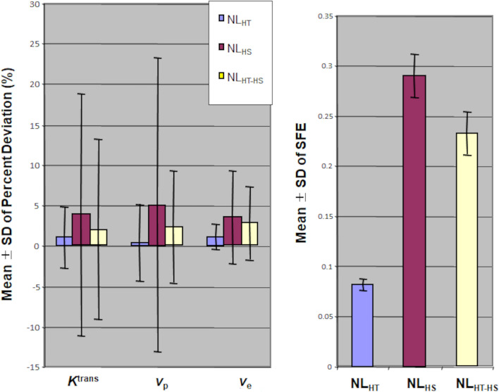
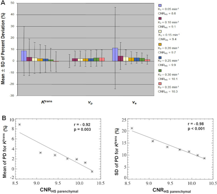
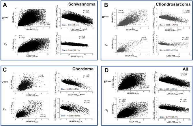
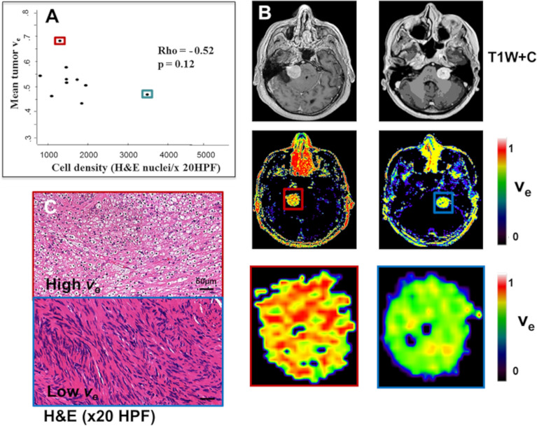
A key limitation of current dynamic contrast enhanced (DCE) MRI techniques is the requirement for full-dose gadolinium-based contrast agent (GBCA) administration. The purpose of this feasibility study was to develop and assess a new low GBCA dose protocol for deriving high-spatial resolution kinetic parameters from brain DCE-MRI. Nineteen patients with intracranial skull base tumours were prospectively imaged at 1.5 T using a single-injection, fixed-volume low GBCA dose, dual temporal resolution interleaved DCE-MRI acquisition. The accuracy of kinetic parameters (v_e, K^trans, v_p) derived using this new low GBCA dose technique was evaluated through both Monte-Carlo simulations (mean percent deviation, PD, of measured from true values) and an in vivo study incorporating comparison with a conventional full-dose GBCA protocol and correlation with histopathological data. The mean PD of data from the interleaved high-temporal-high-spatial resolution approach outperformed use of high-spatial, low temporal resolution datasets alone (p < 0.0001, t-test). Kinetic parameters derived using the low-dose interleaved protocol correlated significantly with parameters derived from a full-dose acquisition (p < 0.001) and demonstrated a significant association with tissue markers of microvessel density (p < 0.05). Our results suggest accurate high-spatial resolution kinetic parameter mapping is feasible with significantly reduced GBCA dose.

Figure 1

Single-injection, low GBCA dose interleaved DCE-MRI protocol. (A) Protocol for the interleaved low GBCA dose high-temporal, high-spatial (HT-HS) interleaved DCE-MRI acquisition. (B) Contrast agent concentration–time course measured from a region-of-interest in the superior sagittal sinus. The arterial phase of the concentration–time course is sampled using fifty dynamic HT frames at the start of the acquisition to allow for accurate discrimination between plasma volume and plasma-leakage effects. Later concentration–time points are sampled using twelve pairs of interleaved low-dose LDHS & LDHT series segments. BL Baseline frame, HS High-spatial, HT High-temporal, LD Low-dose, LDHS Low-dose high-spatial, LDHT low-dose high-temporal.

Figure 2

Monte Carlo simulations to compare parameter accuracy at noise levels resembling the in vivo high-temporal (HT) series, the high-spatial (HS) series, and the interleaved HT-HS series when using low GBCA dose. Mean ± SD of percent deviations (PD) for K^trans, v_p, and v_e, and scaled fitting error from 10,000 Monte Carlo repetitions. Simulated tumour tissue concentration–time curve was synthesized using in vivo pharmacokinetic parameter values from an imaged VS tumour with “true” K^trans = 0.26 min⁻¹, v_p = 0.07, and v_e = 0.5, and converted into signal intensity (SI)-time curves. Values for three different noise levels (NL) shown: (1) a lower noise level resembling the in vivo HT series, NL_HT (= 0.038); (2) a higher noise level resembling the in vivo HS series, NL_HS (= 0.12); (3) a mixed noise level, resembling the in vivo HT-HS interleaved series, NL_HT-HS. Differences in the percent deviations (PD) for K^trans, v_p, and v_e, and SFE between noise levels were compared using paired t-tests.

Figure 3

Monte Carlo simulation of the effects of CNR and K^trans on parameter accuracy when using interleaved HT-HS acquisition. Simulated low-dose HT-HS interleaved tumour SI-time curve was synthesized using a range of ‘true’ K^trans values: K_T 0.05–0.35 min⁻¹; v_p of 0.07; v_e of 0.5, and with the mixed noise level (NL_HT-HS) as used in Fig. 2. (A): Mean ± SD of percent deviations (PD) for K^trans, v_p, and v_e from 10,000 Monte Carlo repetitions at different ‘true’ K^trans values (K_{T :}0.05–0.35 min⁻¹). Increases in ‘true’ K^trans from 0.05 to 0.35 min^-1 resulted in an increase in CNR_HS parenchymal phase (8.6 to 10.3) and a corresponding decrease in the mean PD (increased parameter accuracy) of both K^trans and v_e, with minimal effect on the mean PD accuracy of v_p. (B) Scatterplot demonstrating inverse correlation between CNR levels within the HS parenchymal tissue phase of the interleaved HT-HS derived SI-time curve (CNR_{HS parenchymal phase}) and the mean (left) or SD (right) percent deviations (PD) in estimated K^trans estimates. Correlation reported using Pearson’s product moment correlation coefficient (r). K_T: true K^trans; CNR_{HS parenchymal phase}: contrast-to-noise ratio of the low-dose high-spatial resolution parenchymal tissue phase. For each K^trans setting, CNR_{HS-parenchymal phase} was calculated as (maximum SI of the LDHS parenchymal tissue phase–mean SI of HS baseline)/(SD of HS baseline).

Figure 4

Kinetic parameter maps from a sporadic vestibular schwannoma patient imaged using the single, low GBCA dose interleaved HT-HS DCE-MRI protocol and full GBCA dose (FDHS) acquisition (A) Representative images from a patient with a large left sided sporadic VS imaged using the single-injection low-dose interleaved high-temporal and high-spatial resolution (HT-HS) DCE-MRI acquisition followed by a full dose high-spatial resolution (FDHS) acquisition. Kinetic maps derived using either the low-dose LEGATOS_LDHS method or the full dose LEGATOS_DICE method are shown. Note the increased vascularity around the tumour capsule, visible on both the high-spatial T2W DRIVE acquisition (voxel size = 0.5 × 0.5 × 0.5 × 0.5 mm³) and LEGATOS derived v_p parameter maps ×. (B) Scatterplots demonstrating that for all parameters there was a significant voxelwise correlation between the LEGATOS_LDHS and LEGATOS_DICE derived values (p < 0.001) for the tumour shown in panel A. The overall median voxelwise difference (median % difference) for each of the LEGATOS_LDHS derived parameters with respect to LEGATOS_DICE estimates was− 0.01 (2.26%),− 0.10 min⁻¹ (− 39.2%) and− 0.02 (− 30.0%) for v_e, K^trans and v_p, respectively. For all parameters, the difference/bias in voxelwise LEGATOS_LDHS estimates increased with increasing voxel values (p < 0.001) with regions of high K^trans and v_p on the LEGATOS_DICE maps showing correspondingly lower LEGATOS_LDHS derived parameter values.

Figure 5

Comparison of voxelwise values of K^trans and v_p obtained using the LEGATOS_LDHS and LEGATOS_DICE reconstruction methods. Values shown for all tumour voxels in the schwannoma (panel A, N = 40,116 voxels), chondrosarcoma (panel B, N = 8079 voxels) and chordoma (panel C, N = 3034 voxels) tumour subgroup along with a pooled analysis of tumour voxels across all three tumour groups (panel D, N = 51,229 voxels). Within each panel the voxelwise correlation between LEGATOS_LDHS and LEGATOS_DICE derived estimates for K^trans (top left) and v_p are shown (bottom left). The correlation between the full dose LEGATOS_DICE derived estimates and the voxelwise difference between LEGATOS_LDHS and LEGATOS_DICE estimates is also shown (top and bottom right), along with the median bias or voxelwise difference (median % difference relative to LEGATOS_FDHS estimate) for each of the LEGATOS_LDHS derived parameters. The correlation results are reported using Pearson’s product moment correlation coefficient (r). Voxels with an SFE value > 0.5 and voxel values > 99% centile are excluded from the scatterplots shown.

Figure 6

Comparison of fit error and derived kinetic parameters from different skull base tumours. Representative imaging from a patient with bilateral NF2-related VSs (A), and a patient with chondrosarcoma involving the anterior cranial fossa (B) shown. From left to right: T1W post contrast; parametric v_e map; parametric K^trans map; parametric v_p map; and map of scaled fitting error (SFE). Kinetic maps and maps of SFE derived using either the low GBCA dose LEGATOS_LDHS method or the full GBCA dose LEGATOS_DICE method are shown for each patient. Note the more heterogenous enhancement of the skull base chondrosarcoma (*) relative to the VSs, and the much larger difference in SFE within the chondrosarcoma tumour region between the low-dose and full-dose acquisition.

Figure 7

Comparison of derived v_p and K^trans estimates from the single low-dose DCE-MRI acquisition against tissue-derived vascularity metrics. Representative imaging and histology from a patient with a growing highly vascular VS (top row) and a comparatively less vascular static VS (bottom row) are shown. From left to right: T1W post contrast; parametric K^trans map; parametric v_p map; and immunostains (CD31-brown) demonstrating the comparatively higher microvessel density within the larger growing VS (immunoperoxidase—× 20 HPF).

Figure 8

Comparison of derived v_e estimates from the single low-dose DCE-MRI acquisition against tissue-derived cell density. (A) Inter-tumour scatterplot comparison of LEGATOS_LDHS derived mean tumour v_e estimates against H&E cell density (nuclei/× 20 HPF). Spearman’s rho reported. Data from ten tumours shown. (B) Representative image sections of a VS with high v_e estimates (left) and a VS with low v_e estimates (right). From top: T1W post contrast; parametric v_e map; and magnification image demonstrating voxelwise heterogeneity in v_e estimates across the tumour. (C) Representative haematoxylin and eosin (H&E, × 20 HPF)–stained sections from the tumour with high v_e (top row) and low v_e (bottom row) respectively. Mean tumour v_e values for the VS displayed in Panels B and C are outlined in the scatterplot shown in Panel A with a red and blue box, respectively. HPF High-powered-field.

References

1. O’Connor JPB, Jackson A, Parker GJM, Jayson GC. DCE-MRI biomarkers in the clinical evaluation of antiangiogenic and vascular disrupting agents. Br. J. Cancer. 2007;96:189–195. doi: 10.1038/sj.bjc.6603515. - DOI - PMC - PubMed
1. Li KL, et al. Vascular biomarkers derived from dynamic contrast-enhanced MRI predict response of vestibular schwannoma to antiangiogenic therapy in type 2 neurofibromatosis. Neuro Oncol. 2016;18:275–282. doi: 10.1093/neuonc/nov168. - DOI - PMC - PubMed
1. Lewis D, et al. The microenvironment in sporadic and neurofibromatosis type II–related vestibular schwannoma: The same tumor or different? a comparative imaging and neuropathology study. J. Neurosurg. 2020;134(5):1419–1429. doi: 10.3171/2020.3.jns193230. - DOI - PubMed
1. Lewis D, et al. Inflammation and vascular permeability correlate with growth in sporadic vestibular schwannoma. Neuro Oncol. 2019;21:314–325. doi: 10.1093/neuonc/noy177. - DOI - PMC - PubMed
1. Lewis D, et al. Detection of early changes in the post-radiosurgery vestibular schwannoma microenvironment using multinuclear MRI. Sci. Rep. 2021;11:15712. doi: 10.1038/s41598-021-95022-6. - DOI - PMC - PubMed