Gamma oscillatory complexity conveys behavioral information in hippocampal networks

Abstract

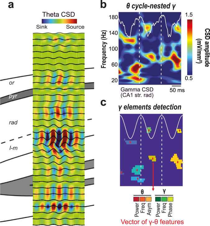
The hippocampus and entorhinal cortex exhibit rich oscillatory patterns critical for cognitive functions. In the hippocampal region CA1, specific gamma-frequency oscillations, timed at different phases of the ongoing theta rhythm, are hypothesized to facilitate the integration of information from varied sources and contribute to distinct cognitive processes. Here, we show that gamma elements -a multidimensional characterization of transient gamma oscillatory episodes- occur at any frequency or phase relative to the ongoing theta rhythm across all CA1 layers in male mice. Despite their low power and stochastic-like nature, individual gamma elements still carry behavior-related information and computational modeling suggests that they reflect neuronal firing. Our findings challenge the idea of rigid gamma sub-bands, showing that behavior shapes ensembles of irregular gamma elements that evolve with learning and depend on hippocampal layers. Widespread gamma diversity, beyond randomness, may thus reflect complexity, likely functional but invisible to classic average-based analyses.

Fig. 1. Detecting and characterizing hippocampal gamma elements.

a Electrodes along the silicon probe were localized in the different layers of the dorsal hippocampus using various indices to identify the hippocampal fissure, including the location of the maximum theta power and of the largest sink in the average theta-triggered CSD. b The gamma composite CSD wavelet spectrogram from each channel was first segmented into theta cycles (two consecutive peaks) from the theta composite signal recorded in the hippocampal fissure (white overlay). c local gamma peaks within the spectrogram were then detected within each theta cycle via a patch detection algorithm. These “gamma elements” were then characterized by extracting a vector of six features: three gamma features (amplitude, frequency, and theta-phase of the gamma element) and three theta features (amplitude, frequency and asymmetry of the coincident theta cycle).

Fig. 2. Hippocampal CA1 layers have overlapping gamma frequency and phase distributions.

a, b Average distributions (mean pdf ± SEM; n = 5 mice) of gamma elements frequency and theta phase for each CA1 layer. Even if significant differences can be found between these distributions (see Supplementary Fig. 5 for details), whatever the layer considered, most of the gamma elements frequency distributions were spread across broad and overlapping ranges of frequencies, encompassing both the classical gamma_S and gamma_M sub-bands definition (full width at half maximum range: oriens (or), 35–97 Hz; pyramidale (pyr), 34–102 Hz; rad, 31–97 Hz; l-m, 38–100 Hz). c A joint representation of the three gamma features emphasizes the haphazard diversity of frequency (radius) and phase (angle) between gamma elements (dots) recorded in both the rad and l-m layers, especially at low amplitude (color: percentile of gamma amplitude). d Average theta-gamma spectrograms, on the contrary, put forward a marked distinction in frequency (and phase in a lesser extent) between the rad (left) and l-m layers (right), suggesting these are respectively largely dominated by gamma_S and gamma_M oscillations. The apparent conflict between the representations in panels c and d is explained by the fact that average spectrograms are dominated by strong amplitude events. This is well visualized by dimensionally reduced representations (e, f) of the six-dimensional vectors describing gamma elements (obtained via a distance-respecting t-SNE algorithm). e Gamma elements from the rad and l-m layers cover similar areas in their joint bidimensional projection. However, the elements with high gamma amplitude (top 30%, dots with darker shade) occupy complementary zones for the two layers. f A color-coding by gamma frequency and phase of the same bidimensional projection shows that these strong elements tend to be: of gamma_M type at theta trough, for the l-m layer; and gamma_S at most phases, for the rad layer. These minorities of strong gamma elements are thus precisely the ones giving rise to rad and l–m average spectrogram peaks in panel (e). Panels b–e: examples from a representative mouse (mouse #3).

Fig. 3. Location during exploration behavior can be decoded from individual gamma elements.

a In our spatial navigation task, reward is located at the end-box of a fixed target arm in a radial maze. The mouse enters the maze from a different arm at every trial. Few trials are performed every day, over several days. Left: example trajectories at different days of learning. Middle: the latency to reward decreases across days (n = 5 mice; mean  ± SEM; Mean X²_(9,49) = 19.342, p = 0.02; Friedman ANOVA), indicating that mice learn the task. Right: In probe trials, no reward is given at the reward location. Mice spend a larger amount of time exploring the former rewarded arm than an opposite one, denoting memory of the reward location (one-tailed t-test, t₍₄₎ = 3.22; p = 0.032). b We trained tree-ensemble classifiers to decode rough location within the maze (target arm, reward RF, other RFs and the remaining locations) from individual gamma elements (three theta and three gamma features, cf. Figure 1b). We also trained alternative classifiers to detect an alternative arm, remote from reward. c Fraction of correctly classified locations, by maze location (colors as in b), for a representative mouse (mouse #3; see Supplementary Fig. 7 for other mice and prediction performance with alternative feature sets and in probe trials). Different classifiers were trained for different depths along the dorsal hippocampal axis (cf. Fig. 1a). Solid lines indicate average performance across all trials (shading, 95% bootstrap c.i.). Performance in detecting target arm, reward and other arms RFs was significantly above chance level (dashed black line) for every anatomical layer.

Fig. 4. Decoding performance is robust, genuine and synergistic.

a Dependence on gamma amplitude. Performance is significantly higher for amplitudes in larger than smaller distribution quartiles (p < 0.002 for target; p < 0.033 for reward), however it remains significant for all but the lowest quartile (p < 0.006 for target Q3). b Dependence on motion speed. Decoding performance for target arm (reward RF) was higher for larger (lower) quartiles of speed (p < 0.004 for target, p < 0.001 for reward), but was significant even for low (high) speed quartiles (target Q3, p < 0.0025; reward Q1, p < 0.011). c In probe trials, decoding performance dropped for both target arm (p < 0.0005) and reward RF (p < 0.0001). Decodability of a generic other arm was lower than for target arm (p < 0.0027), but performance did not drop significantly for reward. d When training classifiers to decode maze location based on reduced input feature sets (only gamma- or theta-related features) decoding performance dropped (e.g., when comparing gamma-only with combined theta and gamma inputs, p < 0.0199 for target arm and p < 0.0014 for reward RF). n = 5 mice; dots, performance averaged over trials and electrodes for different mice; boxes, IQRs and sample mean; whiskers, 95% sample c.i.; *, p < 0.05; **, p < 0.01; ***, p < 0.001 after Bonferroni correction; symbols in brackets denote significance only before Bonferroni correction; one-tailed t-tests of sample vs chance level; two-tailed t-tests between samples.) e Fractions of maze location information conveyed by pair of features were large (bars, averages over mice and feature pairs, grouped by pairs including a specific feature –i.e., n = 15 pairs per feature time n = 5 mice–, for representative rad and l-m channels; whiskers, 95% bootstrap c.i). Mutual information was mostly due to synergy between features, which conveyed little unique or redundant information about location. f Speed accounted for a small fraction only of the variability of individual gamma element features, as revealed by normalized mutual information with speed (n = 5 mice, averages over all mice and features, for representative channels; whiskers, 95% c.i estimated from twice sample standard deviation). We don’t show individual mice values in panels (e) and (f) to avoid figure crowding.

Fig. 5. Relations of gamma elements with behavior depend on training.

a Polar scatter plots of individual gamma elements distribution (as in Fig. 1d), separate for early (days 1–3) and late (days 8–10) trials (n = 5 mice). Wide diversity of gamma elements features is observed at all stages of task learning (here for mouse #3; see Supplementary Figs. 2, 5a and 10 for more details and all mice). Although remaining complex, the distributions are however evolving with learning. b The average performance of decoding maze location (average over all classes, for reference channels in rad and l-m) is higher for late than for early trials, as revealed by boxplots of percent performance improvement for representative channels in both rad and l-m layers (p < 0.013 for rad and p < 0.04 for l-m). c, d We performed cross-classification analyses, training classifiers to decode maze location from gamma ensembles in a range of trials and using them to extract information from other trials in past or future time ranges. c The resulting cross-prediction error matrix (here for a representative rad channel for mouse #3; see Supplementary Fig. 11a for l-m layer and other mice) is asymmetric with respect to the diagonal, indicating that classifiers trained on future trial ranges can decode information from past trial ranges better than in the opposite direction. d This asymmetry is quantitively confirmed by positive percent difference between performances in past-on-future or future-on-past prediction directions (positivity of the increment, p < 0.006 for rad and p < 0.0006 for l-m). In the boxplots of all this figure’s panels dots denote performance improvements for different mice. boxes, IQRs; horizontal line, sample mean; whiskers, 95% sample c.i.; **p < 0.01; ***p < 0.001 after Bonferroni correction. One-tailed t-tests are used for both comparisons of samples with chance level; and between samples.

Fig. 6. Relations of gamma elements with behavior depend on and anatomical layer.

We studied cross-classification between different recording locations and its variations along task learning. a The cross-prediction error matrix (all trials, mouse #3; see Supplementary Fig. 11b for other mice) displays a block structure, indicating that different anatomical locations have alternative types of gamma elements to behavior inter-relations. Hippocampal and non-hippocampal channels form different blocks. Within hippocampus CA1, superior rad and l-m channels belong as well to different sub-blocks. b These anatomically-organized patterns of inter-relations evolve along task learning, as revealed by increased l-m vs rad cross-decodability in late with respect to early stages (percent improvement of cross-prediction performance; p < 0.016 for both l-m-on-rad and rad-on-l-m cross-prediction directions). The improvement in cross-predictability across learning was larger in the l-m-to-rad than in the rad-to-l-m direction (significance of difference, p < 0.042). In the boxplots boxes denote IQRs; horizontal line, sample mean; whiskers, 95% sample c.i.; *, p < 0.05; **, p < 0.01; ***, p < 0.001 after Bonferroni correction. One-tailed t-tests are used for comparisons of: samples with chance; and between samples.

Fig. 7. Large diversity of gamma elements reflects firing patterns at the fringe-of-synchrony.

a We generated simulated LFP-like signals using a computational model of a generic local circuit, generating gamma oscillations and driven by an external theta-modulated input current. The model network included thousands of randomly interconnected spiking excitatory (E) and inhibitory (I) neurons. b Typical raster plot of the spiking activity of selected neurons, with superposed trace of the associated LFP-like signal computed from the model. c Spectrograms of the gamma composite component of simulated LFP-like signals reveal the existence of transient gamma oscillatory events at variable frequencies and phases with a landscape of gamma elements diversity comparable to real recordings. d The diversity and frequency distribution of simulated gamma elements depend on model parameters, such as the density of within-population connectivity K and the average strength of I-to-E synaptic coupling. The parameter-dependency surface of spectral entropy (middle panel) shows that narrower-band oscillations with a more precise frequency occur only when connectivity K is very large (star working point). However, in this case, the level of population synchronization would be unrealistically large (large signal standard deviation; rightmost panel). The degree of synchronization also correlates with the average entropy of individual spike trains (quantifying their temporal irregularity). Entropy is large at the “fringe-of-synchrony” (triangle, circle and square points, corresponding to oscillations with different mean frequencies, cf. Supplementary Fig. 12), when spikes are emitted only every few gamma oscillatory cycles in a random-like fashion, while is low in the more synchronous regime (star point) where synchrony is spike-to-spike. e We constructed a classifier predicting whether a given neuron is emitting a spike or not within a small window centered on a gamma element, whose parameterization is fed as input to the classifier. f, For a subset of more precisely phased neurons (cf. Supplementary Fig. 13), successful decoding was possible, with precision and recall above 70%, indicating that gamma element diversity reflects spiking patterns (for all comparisons with chance level, at least p < 0.023 or smaller). Estimations of Entropy and decoding are performed for E neurons only, as they require binning of spike trains and bin-size have been optimized to E average firing rate. In the boxplot, boxes denote IQRs; horizontal line, sample mean; whiskers, 95% sample c.i.; **, p < 0.01; ***, p < 0.001 after Bonferroni correction. One-tailed t-tests are used for comparisons of samples with chance level.

References

1. Buzsaki G, Draguhn A. Neuronal oscillations in cortical networks. Science. 2004;304:1926–1929. doi: 10.1126/science.1099745. - DOI - PubMed
1. Wang XJ. Neurophysiological and computational principles of cortical rhythms in cognition. Physiol. Rev. 2010;90:1195–1268. doi: 10.1152/physrev.00035.2008. - DOI - PMC - PubMed
1. Gray CM, Konig P, Engel AK, Singer W. Oscillatory responses in cat visual cortex exhibit inter-columnar synchronization which reflects global stimulus properties. Nature. 1989;338:334–337. doi: 10.1038/338334a0. - DOI - PubMed
1. Salazar RF, Dotson NM, Bressler SL, Gray CM. Content-specific fronto-parietal synchronization during visual working memory. Science. 2012;338:1097–1100. doi: 10.1126/science.1224000. - DOI - PMC - PubMed
1. Lisman JE, Jensen O. The theta-gamma neural code. Neuron. 2013;77:1002–1016. doi: 10.1016/j.neuron.2013.03.007. - DOI - PMC - PubMed