

Comparison of individual and ensemble machine learning models for prediction of sulphate levels in untreated and treated Acid Mine Drainage
- PMID: 38429461
- PMCID: PMC10907470
- DOI: 10.1007/s10661-024-12467-8
Comparison of individual and ensemble machine learning models for prediction of sulphate levels in untreated and treated Acid Mine Drainage
Abstract
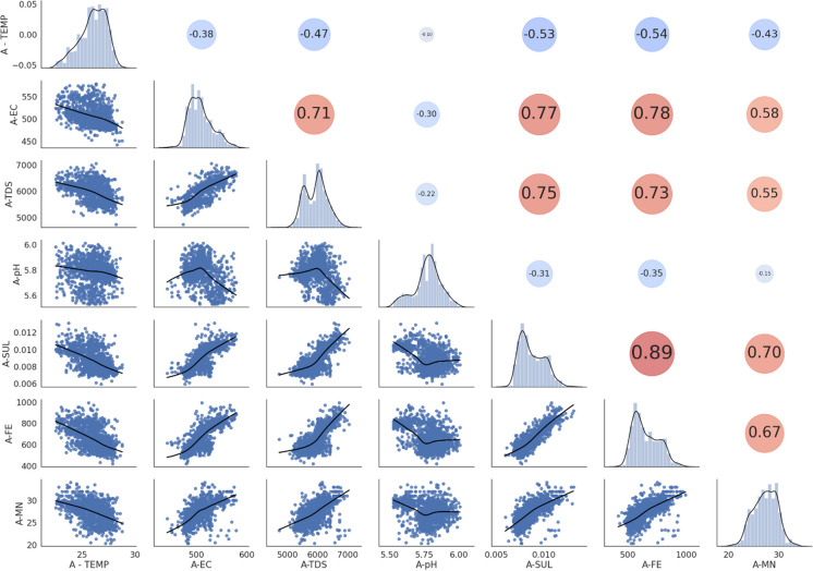
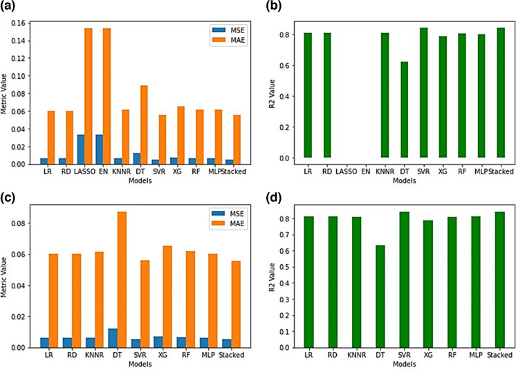
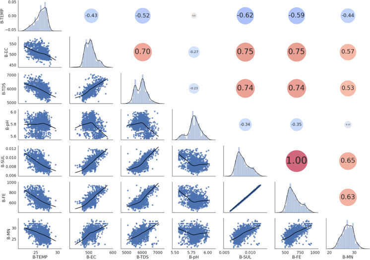
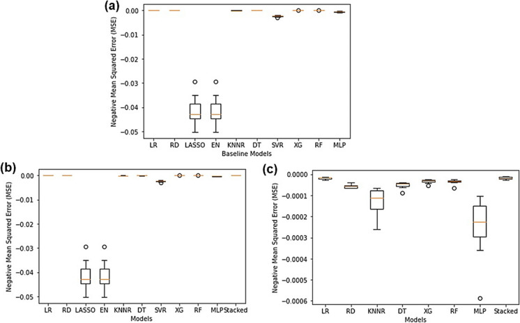
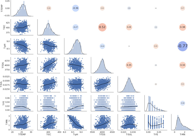
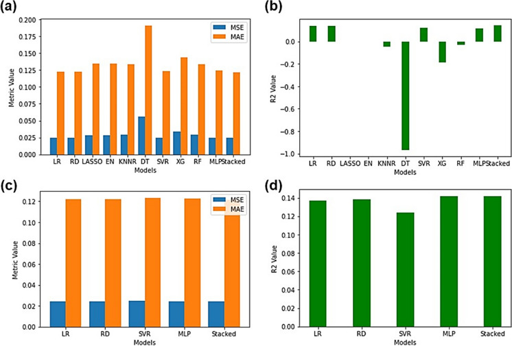
Machine learning was used to provide data for further evaluation of potential extraction of octathiocane (S8), a commercially useful by-product, from Acid Mine Drainage (AMD) by predicting sulphate levels in an AMD water quality dataset. Individual ML regressor models, namely: Linear Regression (LR), Least Absolute Shrinkage and Selection Operator (LASSO), Ridge (RD), Elastic Net (EN), K-Nearest Neighbours (KNN), Support Vector Regression (SVR), Decision Tree (DT), Extreme Gradient Boosting (XGBoost), Random Forest (RF), Multi-Layer Perceptron Artificial Neural Network (MLP) and Stacking Ensemble (SE-ML) combinations of these models were successfully used to predict sulphate levels. A SE-ML regressor trained on untreated AMD which stacked seven of the best-performing individual models and fed them to a LR meta-learner model was found to be the best-performing model with a Mean Squared Error (MSE) of 0.000011, Mean Absolute Error (MAE) of 0.002617 and R2 of 0.9997. Temperature (°C), Total Dissolved Solids (mg/L) and, importantly, iron (mg/L) were highly correlated to sulphate (mg/L) with iron showing a strong positive linear correlation that indicated dissolved products from pyrite oxidation. Ensemble learning (bagging, boosting and stacking) outperformed individual methods due to their combined predictive accuracies. Surprisingly, when comparing SE-ML that combined all models with SE-ML that combined only the best-performing models, there was only a slight difference in model accuracies which indicated that including bad-performing models in the stack had no adverse effect on its predictive performance.
Keywords: Acid Mine Drainage; Environmental chemistry; Machine learning; Regression; Stacking ensemble machine learning; Sulphate.
© 2024. The Author(s).
Conflict of interest statement
The authors declare no competing interests.
Figures


Similar articles
-
Enhancing the Predictive Performance of Molecularly Imprinted Polymer-Based Electrochemical Sensors Using a Stacking Regressor Ensemble of Machine Learning Models.ACS Sens. 2025 Apr 25;10(4):3123-3133. doi: 10.1021/acssensors.5c00364. Epub 2025 Apr 17. ACS Sens. 2025. PMID: 40241481
-
Predictive modeling of blood pressure during hemodialysis: a comparison of linear model, random forest, support vector regression, XGBoost, LASSO regression and ensemble method.Comput Methods Programs Biomed. 2020 Oct;195:105536. doi: 10.1016/j.cmpb.2020.105536. Epub 2020 May 22. Comput Methods Programs Biomed. 2020. PMID: 32485511
-
Using machine learning models to predict the effects of seasonal fluxes on Plesiomonas shigelloides population density.Environ Pollut. 2023 Jan 15;317:120734. doi: 10.1016/j.envpol.2022.120734. Epub 2022 Nov 28. Environ Pollut. 2023. PMID: 36455774
-
Artificial intelligence in clinical care amidst COVID-19 pandemic: A systematic review.Comput Struct Biotechnol J. 2021;19:2833-2850. doi: 10.1016/j.csbj.2021.05.010. Epub 2021 May 7. Comput Struct Biotechnol J. 2021. PMID: 34025952 Free PMC article. Review.
-
An extensive experimental survey of regression methods.Neural Netw. 2019 Mar;111:11-34. doi: 10.1016/j.neunet.2018.12.010. Epub 2018 Dec 21. Neural Netw. 2019. PMID: 30654138 Review.
Cited by
-
An online explainable ensemble machine learning model for predicting epidermal growth factor receptor mutation status in lung adenocarcinoma.Transl Lung Cancer Res. 2025 Jul 31;14(7):2670-2687. doi: 10.21037/tlcr-2025-237. Epub 2025 Jul 28. Transl Lung Cancer Res. 2025. PMID: 40799429 Free PMC article.
References
-
- Alzubi J, Nayyar A, Kumar A. Machine learning from theory to algorithms: An overview. Journal of Physics: Conference Series. 2018;1142:012012. doi: 10.1088/1742-6596/1142/1/012012. - DOI
-
- Arora, S., & Keshari, A. K. (2023). Implementing machine learning algorithm to model reaeration coefficient of urbanized rivers. Environmental Modeling & Assessment10.1007/s10666-023-09895-0
-
- Awad, M., & Khanna, R. (2015). Support vector regression. In Efficient Learning Machines (67–80). Berkeley, CA: Apress. 10.1007/978-1-4302-5990-9_4
MeSH terms
Substances
LinkOut - more resources
Full Text Sources
Research Materials
Miscellaneous
