Biodiversity-production feedback effects lead to intensification traps in agricultural landscapes

Abstract

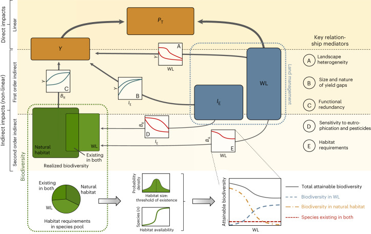
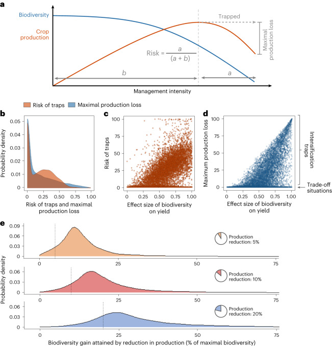
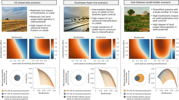
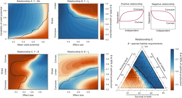
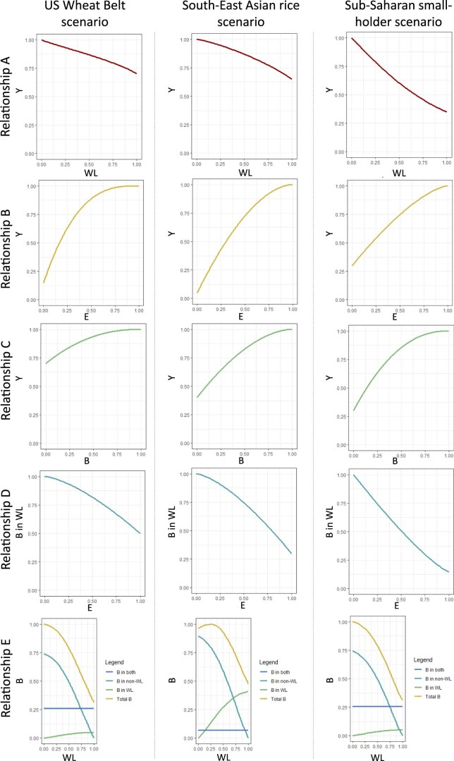
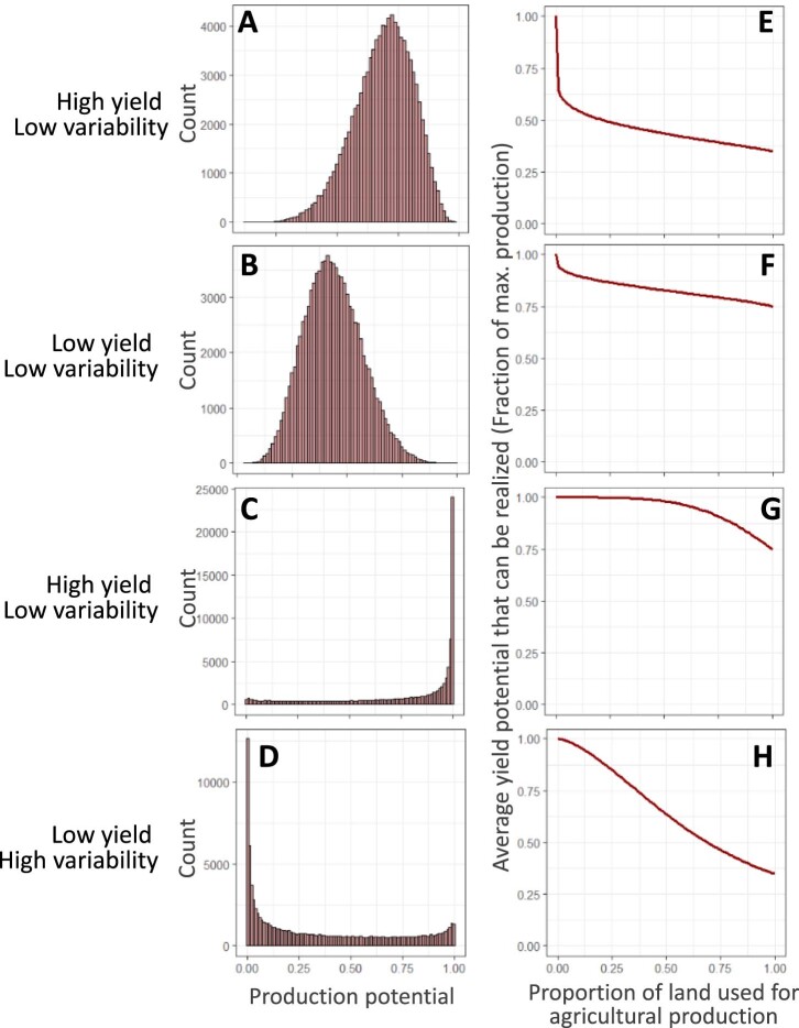
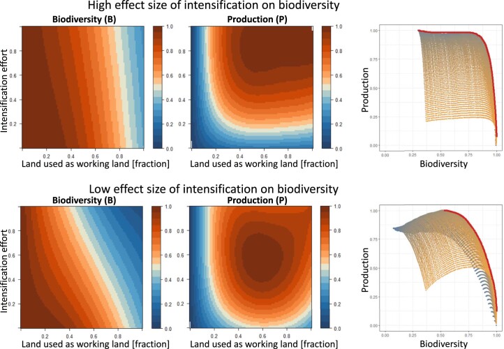
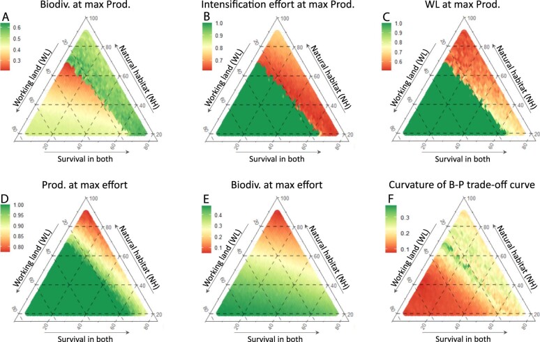
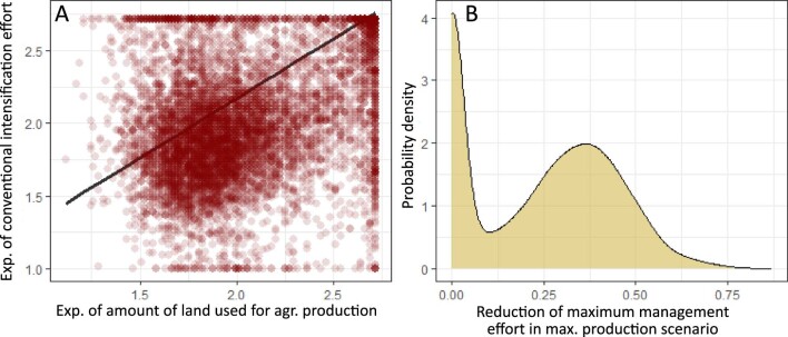
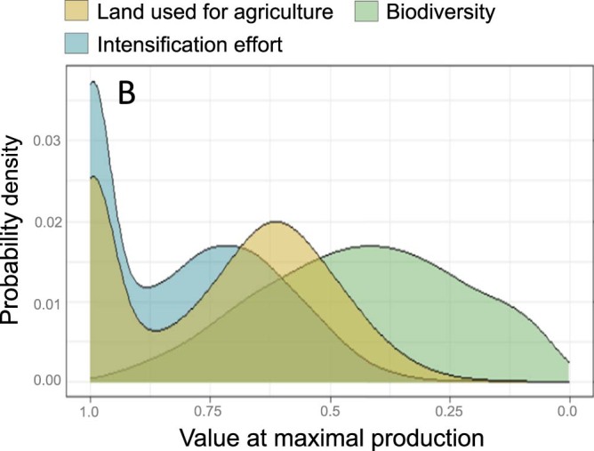
Intensive agriculture with high reliance on pesticides and fertilizers constitutes a major strategy for 'feeding the world'. However, such conventional intensification is linked to diminishing returns and can result in 'intensification traps'-production declines triggered by the negative feedback of biodiversity loss at high input levels. Here we developed a novel framework that accounts for biodiversity feedback on crop yields to evaluate the risk and magnitude of intensification traps. Simulations grounded in systematic literature reviews showed that intensification traps emerge in most landscape types, but to a lesser extent in major cereal production systems. Furthermore, small reductions in maximal production (5-10%) could be frequently transmitted into substantial biodiversity gains, resulting in small-loss large-gain trade-offs prevailing across landscape types. However, sensitivity analyses revealed a strong context dependence of trap emergence, inducing substantial uncertainty in the identification of optimal management at the field scale. Hence, we recommend the development of case-specific safety margins for intensification preventing double losses in biodiversity and food security associated with intensification traps.

Fig. 1. Conceptual overview of five key relationships mediating the impact of land management (blue boxes) on biodiversity (green) and agricultural production (brown).

Land management is characterized by the level of conventional intensification effort (I_E) and the proportion of land used for agriculture (that is, WL). Crop yield, that is, production per area (Y), depends on land-management features directly (plots A and B) and indirectly (C–E) via biodiversity. The effect size (change in the response variable across the range of the predictor) and the shape of these five relationships will vary across landscapes with crop, soil and biotic characteristics and key relationship drivers (listed in the top right). In our framework, the response of the attainable biodiversity (B_A) to changes in land use results from habitat requirements of species in the regional species pool (bottom left) and their required minimum habitat size (bottom centre). Realized biodiversity (B_R) is estimated by subtracting the negative impact of conventional intensification from B_A.

Fig. 2. Characterization of intensification traps in agricultural landscapes.

a, Onset of intensification traps, definition of their risk and their associated maximal production loss. Both risk and maximal production loss are scaled from 0 to 1, with 1 denoting the highest theoretically possible value. b, The distribution of the risk of intensification traps and associated maximal production losses across 10,000 stochastically generated artificial landscapes. Artificial landscapes reflect the variability of the five key relationships (Fig. 1) as recorded in a literature review for each of the model parameters. Parameter values have been range transformed. c,d, The risk of intensification traps (c) and associated maximum yield losses (d) in 10,000 artificial landscapes are dependent on the effect size of biodiversity on yields. Each point represents a landscape. Note that landscapes with high risk (>80% of possible land uses) were occurring in less than 1% of all cases and were driven by situations when biodiversity peaked at intermediate to high contribution of working lands. e, The biodiversity gains attained by decreasing maximum production by 5%, 10% and 20%. Values to the right of the dashed lines indicate greater biodiversity gains than production losses (small-loss large-gain situation).

Fig. 3. Analysis of three selected archetypal landscapes.

Exemplary case studies were chosen as they represent production systems of large importance for global food security that vary in their reliance of yield on biodiversity. In the middle row, responses of biodiversity (left) and agricultural production (right) to changes in management intensity (that is, conventional intensification and the proportion of agricultural land-use) are presented. In the bottom left, maximal attainable biodiversity (dotted circle) is depicted compared with the biodiversity maintained under the land management that leads to the highest agricultural production. Opportunity–cost curves (bottom right), which show the highest attainable biodiversity for each production level, are represented by red lines whereas model scenarios are shown as points coloured based on their conventional intensification effort (high, grey; low, yellow). B, biodiversity; P, production; NH, natural habitat. All axis units are range transformed. Credits, top row: left, josealbafotos/Pixabay; centre, Quangpraha/Pixabay; right, TG23/iStock.

Fig. 4. Systematic sensitivity analysis of how changes in the five key relationships presented in Fig. 1 affect biodiversity–production relationships.

Biodiversity remaining in an agricultural landscape when at least 90% of maximum attainable production is achieved. In five sensitivity analyses (relationships A–E), the model constants describing one of the five key relationships were systematically modified over a predefined range (Supplementary Table 2). The dotted area represents conditions in which intensification traps emerge at maximal management intensity (that is, at maximal conventional intensification and agricultural land expansion). Yield potential in A refers to the highest attainable yield in a given area and was standardized from 0 to 1 in each landscape. Shapes of positive relationships apply to panels B–C, and those of negative relationships, to panel D (top right).

Extended Data Fig. 1. Visualisation of the five key relationships for the three archetypal case-studies.

B stands for biodiversity, WL for working land (that is proportion of landscape used for crop production), Y for yield, non-WL for semi-natural and natural habitat (that is non-working land).

Extended Data Fig. 2. Examples for the distribution of production potential in agricultural landscapes.

A–D display distributions and E–H the respective relationships between average potential yield of used fields and proportion of land used for agriculture (curve is derived from distribution). Parameter settings for mean yield and variance of yields (ranges from 0 to 1) were respectively 0.75 and 0.05 (high yield, low variability), 0.25 and 0.05 (low yield, low variability), 0.75 and 0.5 (high yield, high variability) and 0.25 and 0.5 (low yield, high variability).

Extended Data Fig. 3. The dependency of biodiversity and total production on the intensity of conventional intensification and the extent of working lands in two artificial landscapes.

The two artificial landscapes have been parametrised based on mean literature values for four of the five key relationships and only differ in the parametrisation for relationship D, defining biodiversity responses to conventional intensification. Both landscapes show a linear impact of intensification on biodiversity but landscape 1 (top) was characterised by an effect size of 0.2 whereas the effect size in landscape 2 (bottom) was 0.8. The consequence is that in landscape 1, intensification traps cannot emerge because the negative impact of yield on biodiversity is to small that negative biodiversity feedback-effects on yields overcome the positive effect of intensification on yields. A contrasting situation is found in landscape 2.

Extended Data Fig. 4. Model responses to changes in habitat requirements of species in the regional species pool.

Habitat requirements are defined as inhabiting (i) natural habitat, (ii) working lands or (iii) the ability to survive in both. Displayed as response variables are (a) biodiversity in the scenario with the highest total crop production, (b) the conventional intensification effort in the scenario with the highest production, (c) the proportion of land used as working land in the scenario with the highest production, (d) the production achieved in the scenario with the maximum management effort (that is conventional intensification and agricultural land use are both at their maximum), (e) the biodiversity maintained in the scenario with the maximum management effort and (f) the curvature (that is measure for exponential nature) of biodiversity-production trade-off curves.

Extended Data Fig. 5. The land management options that support maximum total food production in 10000 artificial landscapes.

(a) The relationship between conventional intensification and the amount of land used for agricultural production, which represent the two components of land management considered in our study. Plotted is the land management that leads to maximal food production. Each point represents an individual landscape. The two land management components were positively related. The result of a type 2 regression (R² = 0.36, p < 0.001) is depicted as black line. (b) The distribution of how strongly optimal land management (highest production) deviates from the maximum management scenario (maximal conventional intensification and agricultural land-use). The difference has been calculated as Euclidian distance and is scaled from 0 to 1 with the latter representing the largest possible distance.

Extended Data Fig. 6. Variability of conditions supporting maximal agricultural production.

Displayed are the distributions of biodiversity values, the amount of land used for agricultural production and the conventional intensification effort that support maximum total food production in 10000 artificial landscapes. Biodiversity values are scaled to the maximum biodiversity that can be reached in a landscape.

References

1. Díaz S, et al. Pervasive human-driven decline of life on Earth points to the need for transformative change. Science. 2019;366:eaax3100. doi: 10.1126/science.aax3100. - DOI - PubMed
1. Mason-D’Croz D, et al. Gaps between fruit and vegetable production, demand, and recommended consumption at global and national levels: an integrated modelling study. Lancet Planet. Health. 2019;3:e318–e329. doi: 10.1016/S2542-5196(19)30095-6. - DOI - PMC - PubMed
1. Willett W, et al. Food in the Anthropocene: the EAT–Lancet Commission on healthy diets from sustainable food systems. Lancet. 2019;393:447–492. doi: 10.1016/S0140-6736(18)31788-4. - DOI - PubMed
1. Tilman D, Balzer C, Hill J, Befort BL. Global food demand and the sustainable intensification of agriculture. Proc. Natl Acad. Sci. USA. 2011;108:20260–20264. doi: 10.1073/pnas.1116437108. - DOI - PMC - PubMed
1. Ramankutty N, et al. Trends in global agricultural land use: implications for environmental health and food security. Annu. Rev. Plant Biol. 2018;69:789–815. doi: 10.1146/annurev-arplant-042817-040256. - DOI - PubMed