. 2024 Aug;21(8):1525-1536.
doi: 10.1038/s41592-024-02210-z. Epub 2024 Mar 8.

Learning structural heterogeneity from cryo-electron sub-tomograms with tomoDRGN

Affiliations

Learning structural heterogeneity from cryo-electron sub-tomograms with tomoDRGN

Barrett M Powell et al. Nat Methods. 2024 Aug.

Abstract

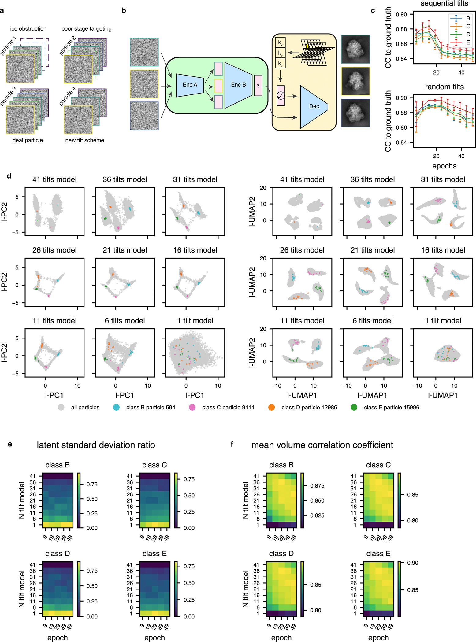
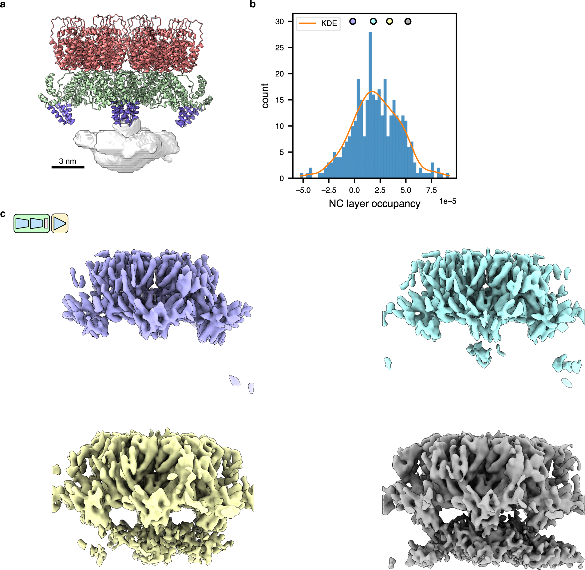
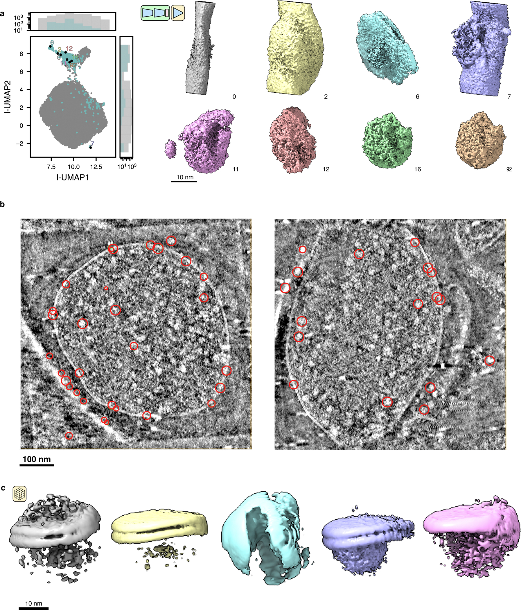
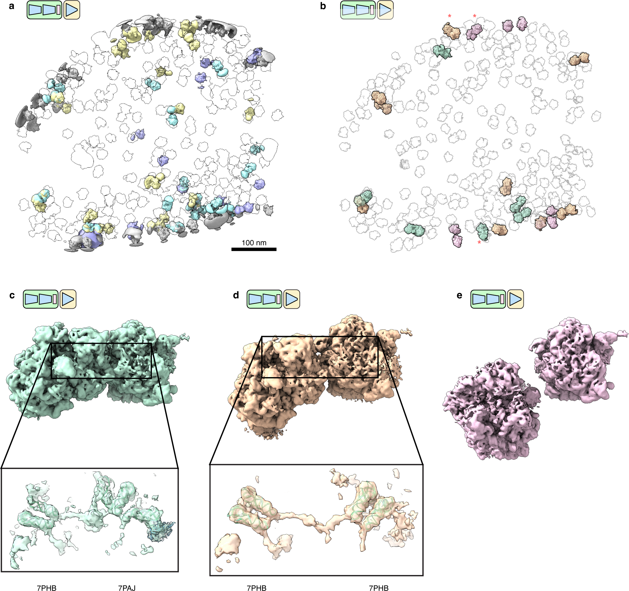
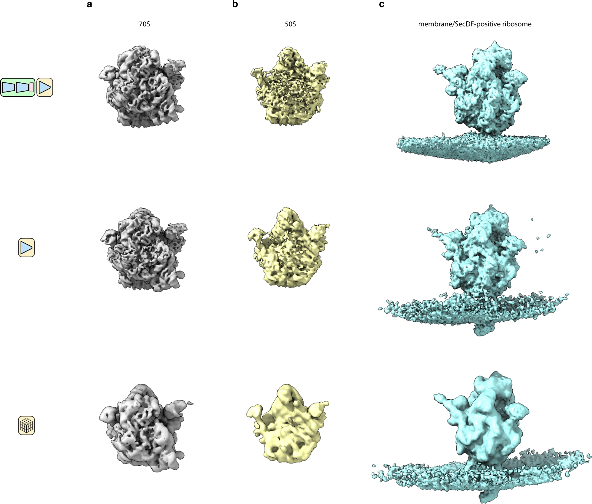
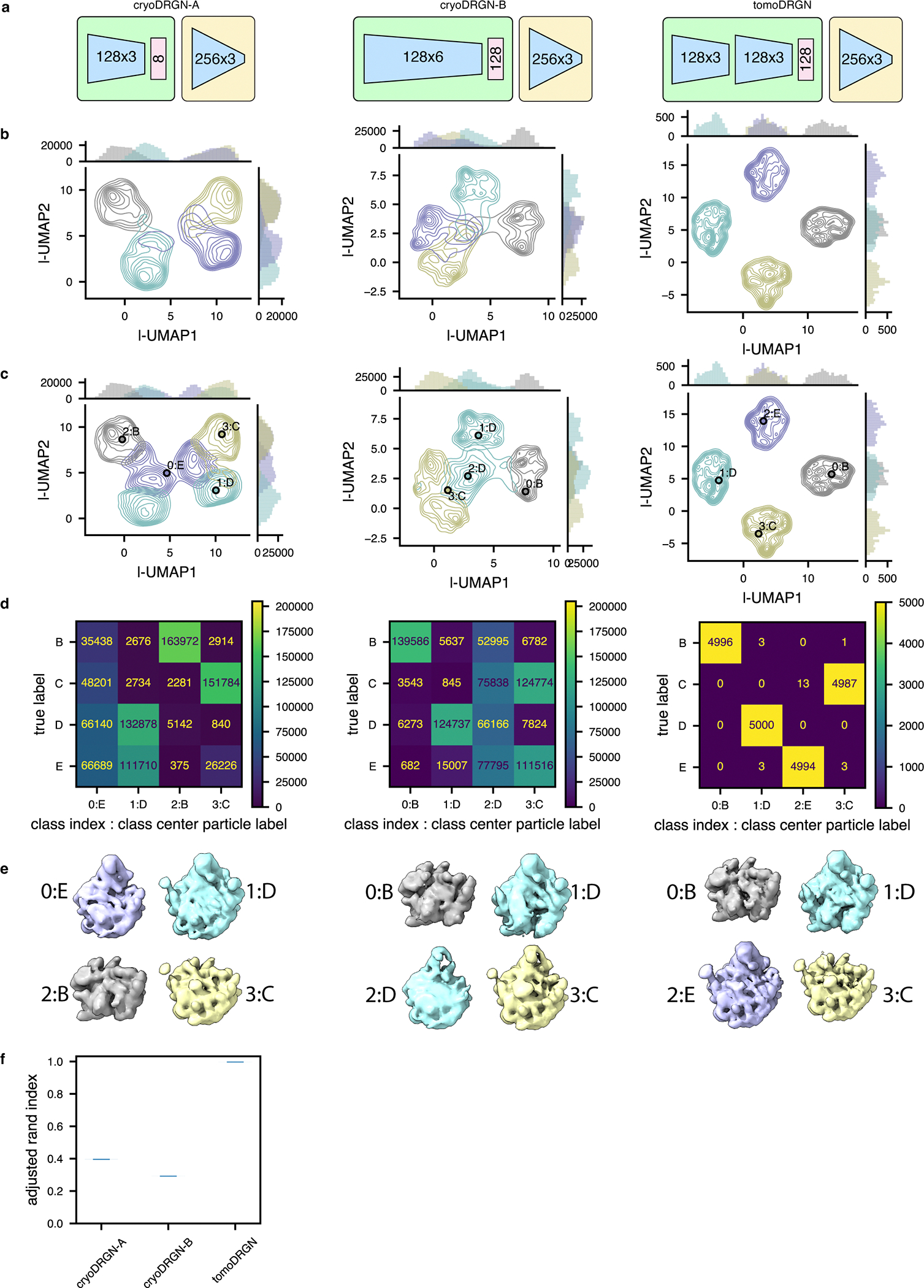
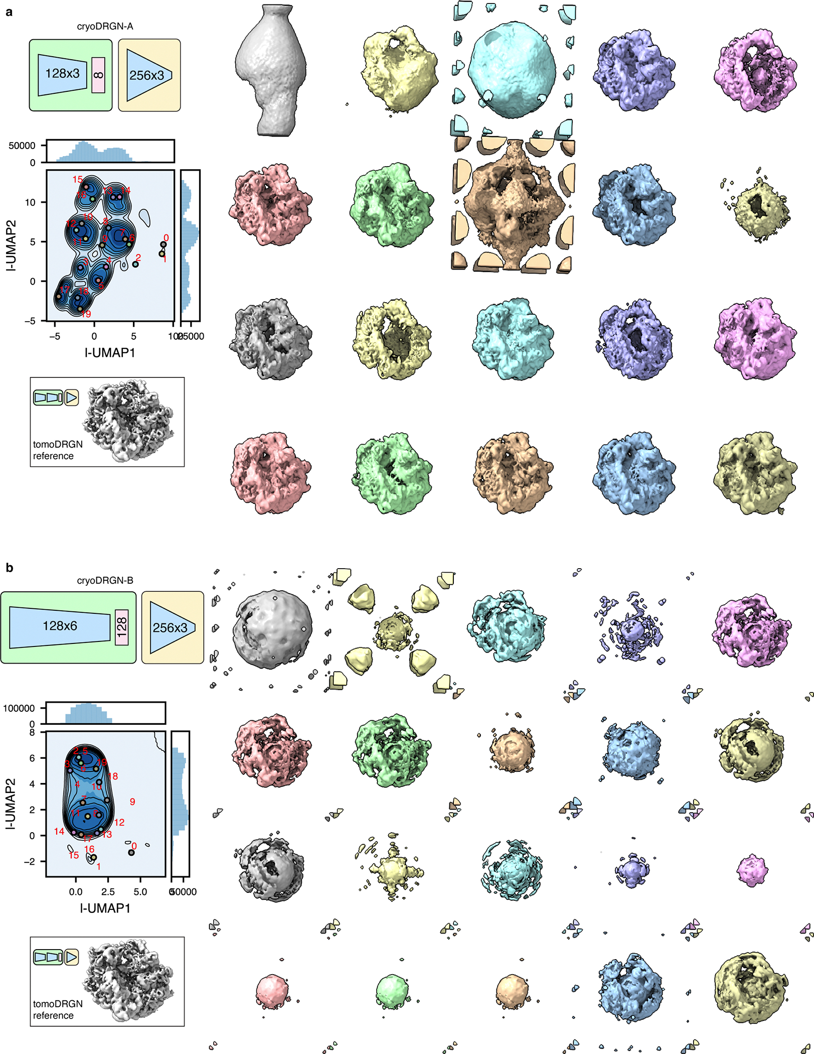
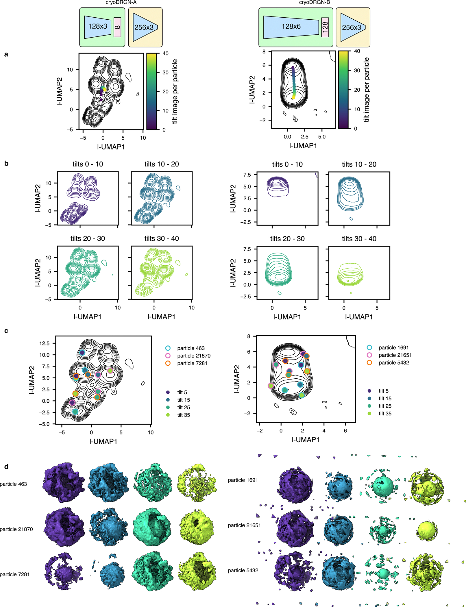
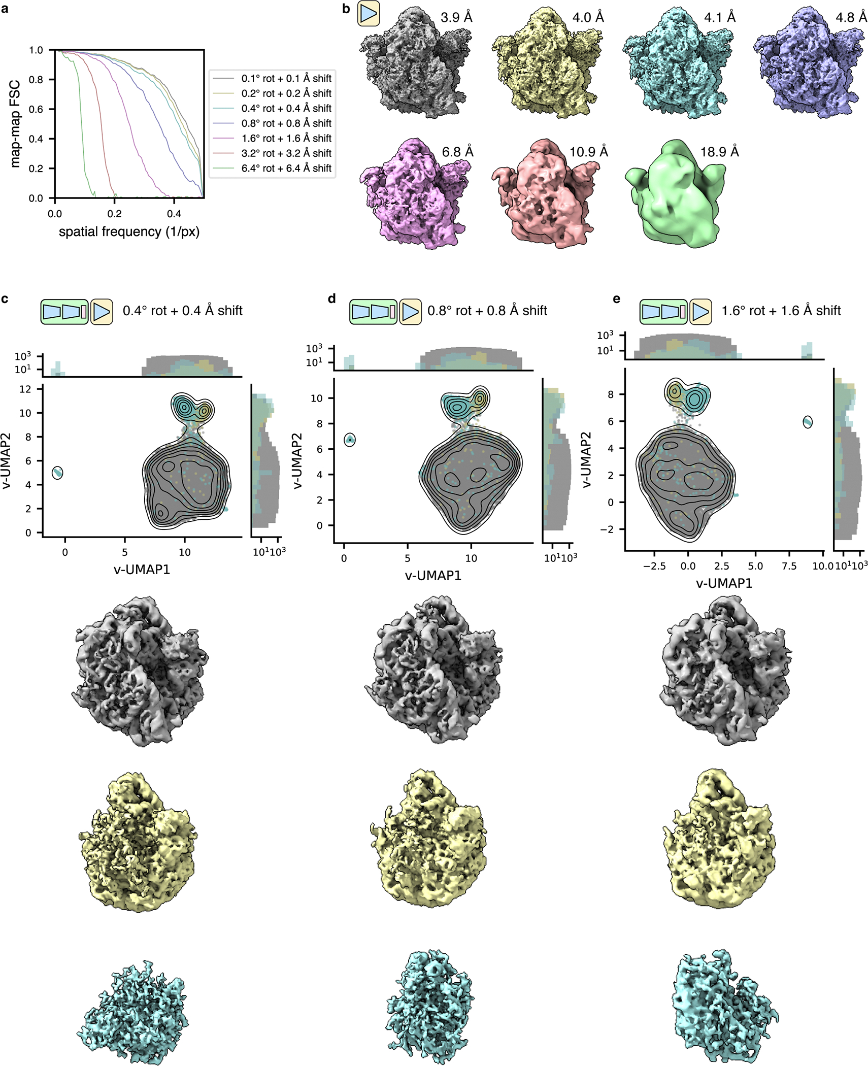
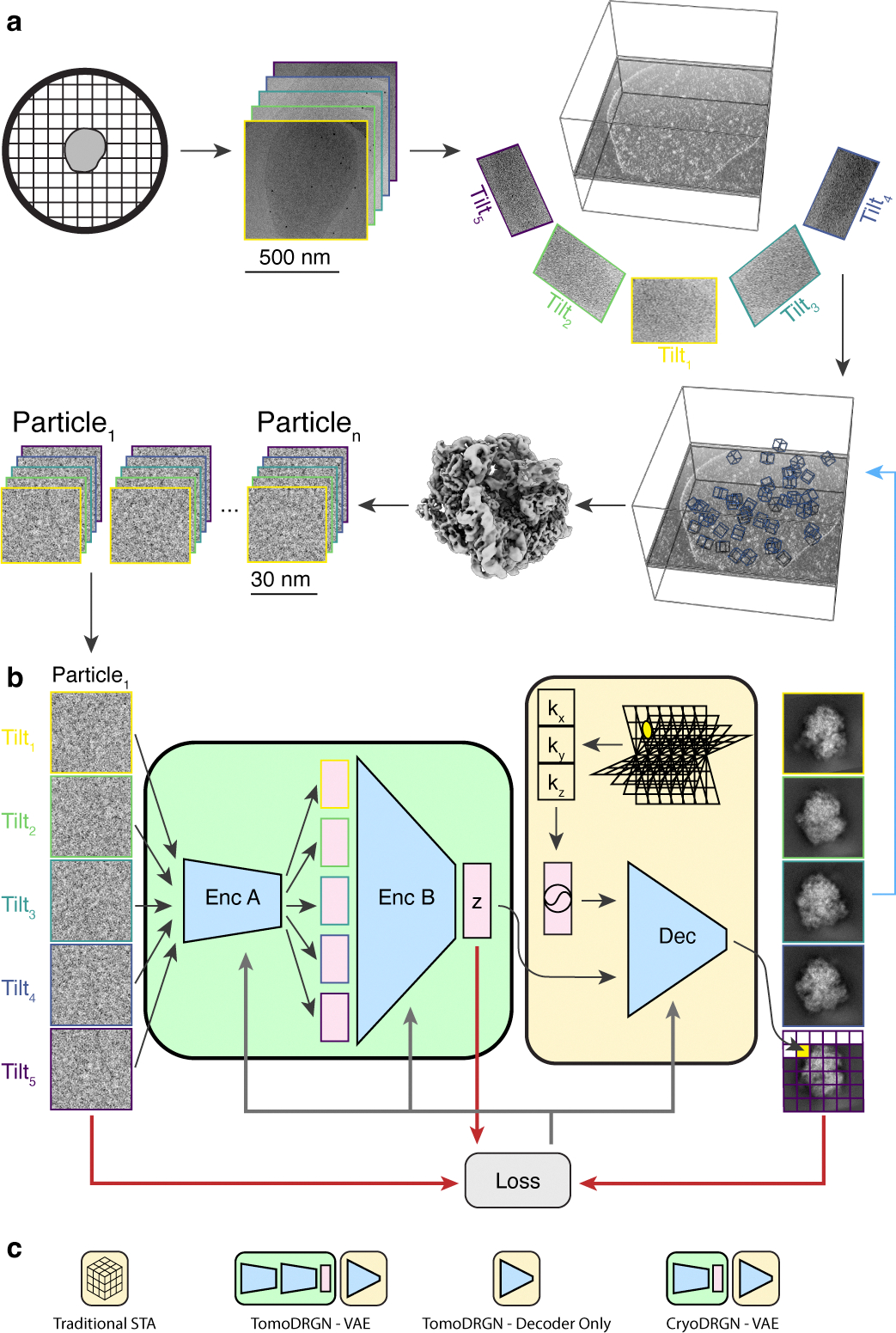
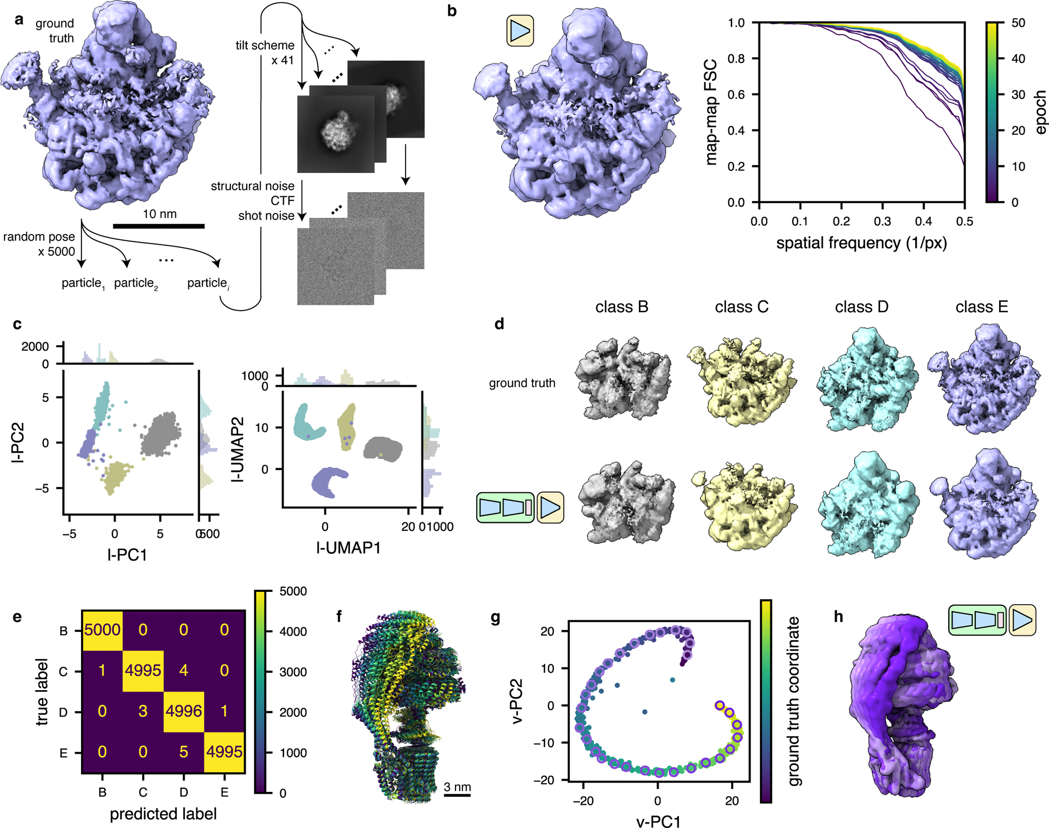
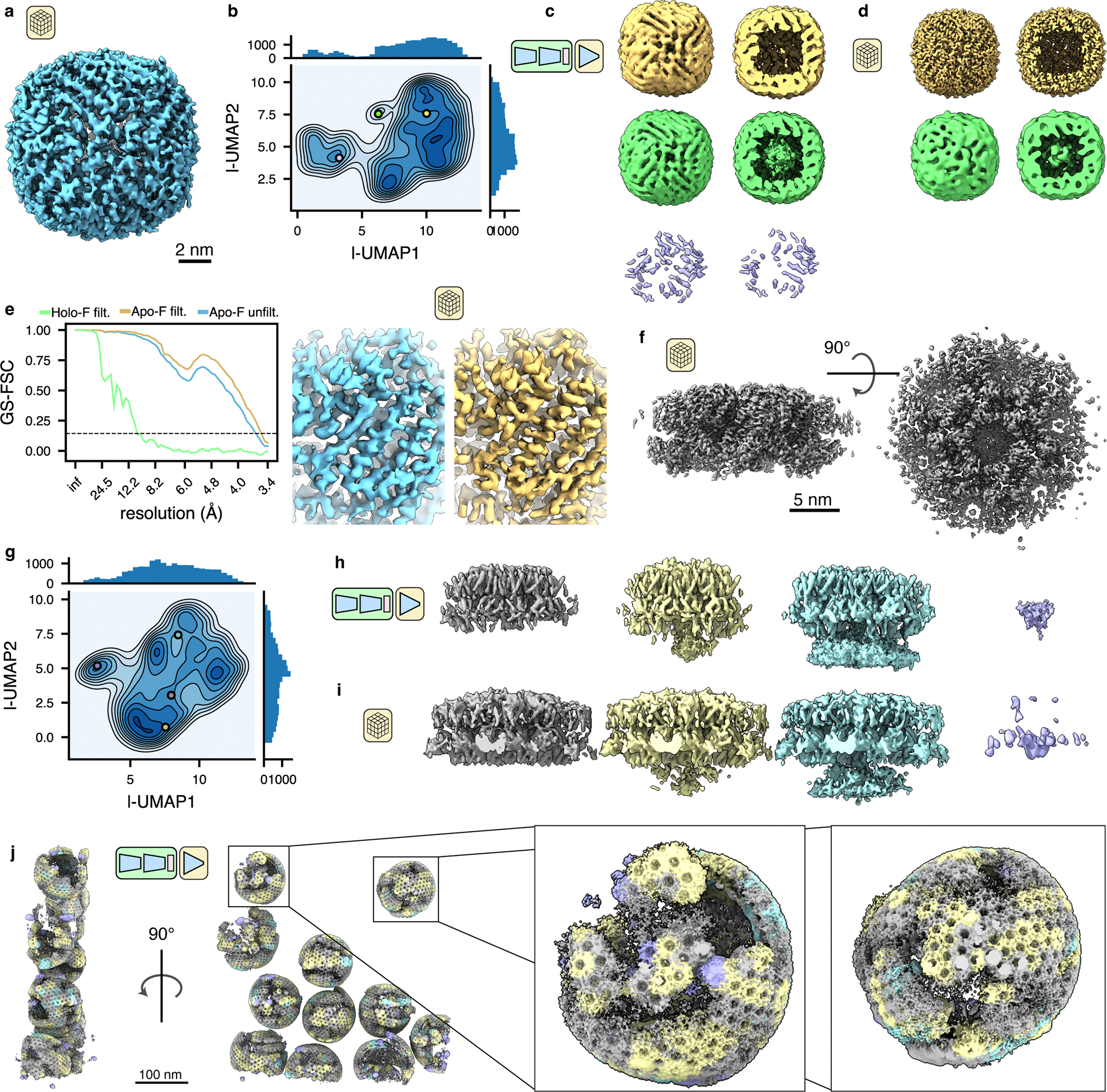
Cryo-electron tomography (cryo-ET) enables observation of macromolecular complexes in their native, spatially contextualized cellular environment. Cryo-ET processing software to visualize such complexes at nanometer resolution via iterative alignment and averaging are well developed but rely upon assumptions of structural homogeneity among the complexes of interest. Recently developed tools allow for some assessment of structural diversity but have limited capacity to represent highly heterogeneous structures, including those undergoing continuous conformational changes. Here we extend the highly expressive cryoDRGN (Deep Reconstructing Generative Networks) deep learning architecture, originally created for single-particle cryo-electron microscopy analysis, to cryo-ET. Our new tool, tomoDRGN, learns a continuous low-dimensional representation of structural heterogeneity in cryo-ET datasets while also learning to reconstruct heterogeneous structural ensembles supported by the underlying data. Using simulated and experimental data, we describe and benchmark architectural choices within tomoDRGN that are uniquely necessitated and enabled by cryo-ET. We additionally illustrate tomoDRGN's efficacy in analyzing diverse datasets, using it to reveal high-level organization of human immunodeficiency virus (HIV) capsid complexes assembled in virus-like particles and to resolve extensive structural heterogeneity among ribosomes imaged in situ.


Conflict of interest statement

COMPETING INTERESTS STATEMENT

The authors declare no competing interests.

Figures

Extended Data Fig. 1
Extended Data Fig. 1. Efficient model training on a weighted subset of pixels improves reconstruction quality and compute performance.
(a) Graphical overview of the dose filtering scheme (applied upstream of the decoder) and dose and tilt weighting scheme (applied during reconstruction error calculation) for a single representative tilt image. Filtering: the fixed optimal exposure curve is used to determine which spatial frequencies will be considered as a function of dose; the decoder processes only Fourier lattice coordinates within this mask (green lattice circle). Weighting: the squared error of the reconstructed Fourier slice is weighted per-frequency by the exposure-dependent amplitude attenuation curve and per-slice by the cosine of the corresponding stage tilt angle, before backpropagation of the mean squared error (red arrows). (b) Relative weight of each tilt image assigned to a particle’s reconstruction error during model training as a function of spatial frequencies (x-axis), and tilt and dose, which are colored yellow to blue from low-to-high dose and tilt angle, assuming a dose symmetric tilt scheme (Hagen, Wan et al. 2017). Note that dose-filtering is applied upstream of the illustrated reconstruction weights. (c) Map-map FSC of simulated class E large ribosomal subunit volumes (Davis, Tan et al. 2016) compared to tomoDRGN homogeneous network reconstructions in the presence or absence of the weighting or masking schemes at varying box and pixel sizes. (d) Spatial frequencies corresponding to FSC=0.5 map-map correlation with the ground truth volume plotted against wall time for model training. (e) Final tomoDRGN reconstructed volumes (left and center) and ground truth volumes (right) in the presence or absence of the weighting or masking schemes at box and pixel sizes assessed in panels (c) and (d).
Extended Data Fig. 2
Extended Data Fig. 2. Random selection of tilts per epoch allows flexible and robust model training for datasets with non-uniform numbers of tilt-images per particle.
(a) Graphical summary of a dataset with non-uniform numbers of tilt images per particle. Here, the minimum number of tilt images for any particle is 3. (b) Corresponding tomoDRGN network architecture for random sampling and ordering of 3 tilt images per particle. (c) Mean per-class volumetric correlation coefficient for identical tomoDRGN models trained on 41 sequentially sampled tilts (top) or 41 randomly sampled tilts (bottom). At 5 epoch intervals, 25 random volumes were generated from each class for correlation coefficient calculation to ground truth ribosome assembly intermediate volumes (classes B-E). Error bars denote standard error of the mean CC. (d) Nine tomoDRGN models with identical architectures were trained with the indicated number of tilts sampled per particle (total available tilts = 41). PCA (left) and UMAP (right) dimensionality reduction of each final epoch’s latent embeddings. Once trained, up to 10 randomly sampled and permuted tilt images for one representative particle from each volume class were embedded using the corresponding pretrained tomoDRGN model and are superimposed as colored points. Note increased dispersion of colored points as number of tilts sampled during training decreased. (e) For each ribosomal large subunit class (B-E), 25 particles were randomly selected and up to 10 subsets of their tilt images were randomly sampled and permuted as in (d). In the heatmap, row indices refer to models trained in (d) using different numbers of sampled tilts (1–41), and columns denote epochs of training with that model. For each particle, each tilt subset was evaluated with the corresponding tomoDRGN model and the ratio of standard deviations of each particle’s 10 latent embeddings to all particles’ latent embeddings was calculated. The mean ratio across all particles, which measures the dispersion of encoder embeddings, is plotted per ribosomal LSU class. Here, lower dispersion indicates better performance. (f) Particles and tilt subsets were selected as in (e). At each indicated epoch of training, the corresponding tomoDRGN model was used to generate volumes for each particle’s tilt subsets. For each such volume, the correlation coefficient was calculated between that volume and the corresponding ground truth volume. The mean across all particles at each epoch for each model is shown as a heatmap per ribosomal LSU class. Here, higher CC indicates improved performance.
Extended Data Fig. 3
Extended Data Fig. 3. TomoDRGN and MAVEn identify structural variations within HIV Gag lattice.
(a) Mask used for MAVEn-based occupancy analysis of NC layer density (gray, translucent). PDB: 5L93 is shown for reference, with CA-NTD colored salmon, CA-CTD colored green, and CA-SP1 helix colored purple. (b) Histogram and kernel density estimate of NC layer occupancy across 500 volumes sampled from the trained tomoDRGN model, excluding junk particles (see Fig 3g). (c) Representative volumes sampling along the NC occupancy histogram, colored as indicated in (b). Volumes are rendered at constant isosurface and same pose as in (a).
Extended Data Fig. 4
Extended Data Fig. 4. TomoDRGN identifies non-ribosomal particles picked from EMPIAR-10499 tomograms.
(a) Latent UMAP and corresponding sampled volumes from tomoDRGN heterogeneous network training from Fig. 5a. Eight representative non-ribosomal particles identified through manual inspection of k=100 k-means clustering of latent space are rendered at a constant isosurface and pose. (b) Two tomograms are shown in slice view using Cube (https://github.com/dtegunov/cube) with locations of particles labeled as non-ribosomal annotated within each tomogram. (c) RELION3-based multiclass (k=5) ab initio sub-tomogram volume generation using particles annotated as non-ribosomal via tomoDRGN (n=1,310).
Extended Data Fig. 5
Extended Data Fig. 5. TomoDRGN visualizes structurally heterogeneous disomes.
(a) An EMPIAR-10499 tomogram reconstructed with tomoDRGN intermolecular volumes. Volumes were generated for each ribosome using the trained intermolecular tomoDRGN model, colored as in Fig. 6a, and positioned correspondingly in the source tomogram. Transparent ribosomes correspond to free 50S and 70S ribosomes as annotated in Fig. 6a. (b) The same tomogram as in panel (a) reconstructed with tomoDRGN intramolecular volumes. Volumes were generated for each ribosome using the trained intramolecular tomoDRGN model (Fig 5d). Pairs of volumes that were colored as disomes or trisomes and that exhibited mutually overlapping main and adjacent monosomes when mapped back to the tomogram in panel (a) were combined in ChimeraX (n=21 disomes). Disomes are colored by manual classification into three classes with representative volumes indicated with asterisks and shown in panels (c-e). (c) A representative disome exhibiting continuous mRNA density between the two monosomes, including unattributed globular density along the mRNA (n=7 disomes). Density of each monosome fit by the indicated atomic model, excluding tRNA, mRNA, and elongation factors, has been removed using ChimeraX’s zone functionality (Inset). (d) A representative disome exhibiting continuous mRNA density between the two monosomes (n=9 disomes). Inset as in panel (c). (e) A representative ribosome pair with no apparent structural contact between the two monosomes (n=5 disomes). Inset as in panel (c).
Extended Data Fig. 6
Extended Data Fig. 6. Comparison of tomoDRGN-generated volumes to traditional sub-tomogram averaged volumes.
Comparison of volumes generated by a full tomoDRGN network (row 1), an isolated decoder neural network (row 2), or traditional sub-tomogram averaging (row 3). A full tomoDRGN network was trained on the heterogeneous ribosomal particle stack (row 1, n=20,981, see Figs. 5d and 6a) and representative volumes are depicted. Separate tomoDRGN homogeneous decoder networks were trained on one of three homogeneous substacks corresponding to (a) 70S particles (n=20,129); (b) 50S particles (n=852); or (c) SecDF-positive ribosomes (n=380). Traditional STA was also performed on each of these three particles stacks.
Extended Data Fig. 7
Extended Data Fig. 7. CryoDRGN fails to consistently encode structural heterogeneity using a simulated tilt series dataset.
(a) Schematic of two cryoDRGN network architectures that were tested, and the tomoDRGN architecture used in Fig. 2c–e. Each model was trained using the same simulated dataset of ribosome large subunit assembly classes B-E (Davis, Tan et al. 2016) consisting of 41 tilt images for each of 5,000 particles for each of the four assembly states and thus the dataset was treated by cryoDRGN as n=820,000 images (see Methods). (b) UMAP of final epoch latent embeddings of each particle image, with kernel density estimates independently estimated and plotted for each of the four ground truth assembly states. (c) UMAP of final epoch latent embedding with k=4 k-means latent classification of the resulting latent space. KDEs were independently estimated and plotted for each of the four k-means classes. The predicted labels are annotated by both the k-means class index (0–3) and corresponding ground truth class label (B-E) of the central particle within each k-means class. (d) Confusion matrix of ground truth class labels versus k=4 k-means latent classification. (e) Volumes sampled at the k=4 k-means cluster centers illustrated in (c). Volumes are annotated by the k-means class index and ground truth class label and colored by the ground truth class label. (f) Violin plot of consistency of k=4 k-means clustering of each model by Adjusted Rand Index (Hubert and Arabie 1985) (n = 100 randomly seeded initializations, higher values correspond to greater fidelity to ground truth classification).
Extended Data Fig. 8
Extended Data Fig. 8. CryoDRGN learns errant structural heterogeneity in an exemplar tomographic dataset.
Two cryoDRGN models (a, b) were trained on the unfiltered particle stack of Mycoplasma pneumoniae ribosomes from Fig. 5a (n = 22,291 particles, treated as n = 913,931 images). The latent space is shown as a KDE plot following UMAP dimensionality reduction, with k=20 k-means class center particles annotated (left) and corresponding volumes visualized (right). Note that many putative 70S particles lack density in the particle core. A reference 70S volume sampled from tomoDRGN’s model in Fig. 5a is shown in the same pose for comparison.
Extended Data Fig. 9
Extended Data Fig. 9. CryoDRGN’s learned latent space embeddings exhibit undesirable correlations with tilt image index.
(a) Two cryoDRGN models were tested on the unfiltered particle stack of Mycoplasma pneumoniae ribosomes from Fig. 5a. The latent space is shown as a KDE plot following UMAP dimensionality reduction. The latent embeddings were binned by the tilt image index, and the median value across each bin is annotated. (b) KDEs from panel A replotted after binning by tilt image index quartiles. (c) KDEs from panel A with annotated positions corresponding to three representative particles evaluated using their 5th, 15th, 25th, or 35th tilt images. (d) Volumes generated from cryoDRGN using the latent embeddings highlighted in panel C.
Extended Data Fig. 10
Extended Data Fig. 10. Assessment of tomoDRGN sensitivity to pose accuracy.
(a) The unfiltered stack of EMPIAR-10499 ribosomes in situ from Fig. 5a was used to train a series of tomoDRGN decoder-only models with increasing levels of random perturbations from STA-derived, “ground truth” rotation and translation poses (see Methods). The resulting map-map FSC curves against the STA ribosomal reconstruction are shown. (b) Final tomoDRGN decoder-only reconstructed volumes corresponding to the FSC curves shown in (a). Volumes are lowpass filtered to the resolution where their map-map FSC to the STA ribosomal reconstruction crossed 0.5. (c, d, e) UMAP of first 128 principal components of volume ensembles consisting of volumes generated for every particle, using tomoDRGN models trained on EMPIAR-10499 unfiltered ribosome stacks with indicated levels of pose perturbation. Particles annotated as 70S, 50S, and NR are colored as in Fig. 5c, with representative volumes of each class shown below. Note that NR particles are expected to be structurally diverse.
Figure 1:
Figure 1:. A neural network architecture to analyze structurally heterogeneous particles imaged by cryo-ET.
(a) A typical sample and data processing workflow to produce tomoDRGN inputs. The sample (e.g., a bacterial cell) is applied to a grid, plunge frozen, and optionally thinned. A series of TEM images of a target region are collected at different stage tilts. A tomographic volume is reconstructed using weighted back-projection of all tilt images. Instances of the target particle are identified (blue boxes) and extracted as 3-D voxel arrays. Iterative sub-tomogram averaging (STA) is used to reconstruct a consensus density map. Per-particle 2-D tilt images are then re-extracted from the source tilt series images and parameters (e.g. pose, defocus, etc.) estimated from STA are associated with the images. (b) The tomoDRGN network architecture and training design. Each particle’s set of tilt images are independently passed through Encoder A, then jointly passed through Encoder B, thereby mapping all tilt images of a particle to one embedding (z) in a low dimensionality latent space. The decoder network (Dec) uses the latent embedding and a featurized voxel coordinate to decode a corresponding set of images pixel-by-pixel. Note that the decoder can learn a homogeneous structure by excluding the encoder module (green). The network is trained using a loss function (grey arrows) that depends on the input images, reconstructed images, and z (red arrows). (c) Graphical signposts for volumes generated or analyzed by different reconstruction tools. These signposts are used throughout this manuscript when volumes are displayed to clarify how they were generated.
Figure 2:
Figure 2:. TomoDRGN recovers compositional and conformational heterogeneity in simulated datasets.
(a) Illustration of the method used to simulate tilt series particle stacks corresponding to four assembly states (B-E) of the bacterial large ribosomal subunit. (b) Left, a tomoDRGN homogeneous network reconstruction of the simulated class E dataset after 50 epochs of training using simulated images with a Nyquist resolution limit of 7.1 Å. Right, Fourier Shell Correlation between the tomoDRGN reconstruction and the ground truth volume at each of 50 epochs of training (purple to yellow). (c) First two principal components (left) and UMAP embeddings (right) of tomoDRGN latent space when trained on the simulated four class dataset, colored by k=4 k-means classification of latent space. (d) Ground truth ribosomal volumes (top) and corresponding tomoDRGN-reconstructed volumes (bottom) sampled from the median latent encoding of each of the k=4 k-means classes in (c). (e) Confusion matrix of k-means clustering class labels from (c) against ground truth class labels. (f) Superposition of yeast mitochondrial ATP synthase structures undergoing conformational changes during ATP hydrolysis. Maps are colored purple to yellow along the simulated reaction coordinate. (g) Voxel-based principal component analysis (vPCA) of 500 tomoDRGN-generated volumes sampled from a tomoDRGN model trained on the simulated ATP synthase dataset from panel (f). Points corresponding to each of the 500 tomoDRGN-generated volumes are colored according to their position along the simulated ground-truth reaction coordinate (see color scale). A subset of 30 such maps are sampled along the trajectory and outlined with a pink-to-purple color gradient, and these maps are presented in Supplementary Movie 1. (h) Superposition of 6 tomoDRGN-generated volumes sampled down the continuous coordinate visualized in panel (g) and colored accordingly.
Figure 3:
Figure 3:. TomoDRGN finds residual heterogeneity within primarily-homogeneous purified particles.
(a) Consensus STA apoferritin structure refined with C1 symmetry (EMPIAR-10491, n = 25,381 particles). (b) UMAP dimensionality reduction of tomoDRGN latent encodings from training on apoferritin dataset. (c) Three volumes generated from tomoDRGN latent encodings sampled as indicated in (b) and rendered in their entirety (left) or clipped in plane (right). (d) Consensus STA reconstructions of apoferritin (n = 16,576 particles; top) and iron-loaded ferritin (n = 542 particles; bottom) from multi-species refinement in M with C1 symmetry using tomoDRGN’s particle classifications, rendered at constant isosurface as in (c). (e) Gold standard FSC curves between half-maps from the final round of M refinement with C1 symmetry for unfiltered apoferritin particles (blue) and filtered apoferritin (yellow) and iron-loaded ferritin particles (green) (left). Example of local density quality before (blue) and after (yellow) tomoDRGN particle filtering of apoferritin particles (right). (f) Consensus STA HIV gag structure refined with C1 symmetry (EMPIAR-10164, n=18,325 particles). (g) UMAP dimensionality reduction of tomoDRGN latent encodings from training on HIV Gag dataset. (h) Four illustrative volumes generated from tomoDRGN latent encodings sampled as indicated in (g). Note increasing density corresponding to the lower NC layer in the yellow and cyan maps relative to that in gray. (i) Weighted back-projection reconstructions of isolated structural classes using tomoDRGN’s particle classifications (from left to right, n = 11,449 particles, 3,546 particles, 1,444 particles, and 1,674 particle), rendered at constant isosurface. (j) An EMPIAR-10164 tomogram reconstructed with tomoDRGN. Volumes were generated for each Gag hexamer using tomoDRGN, colored as in (h, i), and positioned correspondingly in the source tomogram. Inset highlights two representative VLPs.
Figure 4:
Figure 4:. TomoDRGN resolves high resolution features from sub-tomograms collected in situ.
(a) M. pneumonaie ribosomal volume obtained from traditional STA processing (n=22,291 particles imaged in situ). (b) Gold standard FSC curve between half-maps for the volume shown in (a). The second y-axis depicts a histogram of local resolution throughout the map. (c) TomoDRGN homogeneous reconstruction of the particles used for the reconstruction in (a), lowpass filtered to 3.5Å. (d) Map-to-map FSC of three tomoDRGN homogeneous reconstructions of the particle stack in (a) at indicated box and pixel sizes against corresponding STA volumes. Circles denote the Nyquist limit for each particle stack. (e) Local density maps, lowpass filtered at 3.5Å, resulting from tomoDRGN homogeneous reconstruction in (c).
Figure 5:
Figure 5:. TomoDRGN uncovers structural heterogeneity in ribosomes imaged in situ
(a) UMAP of tomoDRGN latent embeddings (n=22,291 particles) shown as gray kernel density estimate (KDE), overlaid with scatter plot depicting latent embedding locations of large-ribosomal-subunit-only (yellow) or non-ribosomal particles (blue) identified via k=100 k-means classification of latent space and manual inspection of the 100 related volumes. Representative volumes generated from latent embeddings annotated as 70S, 50S, or non-ribosomal (NR) also depicted. (b) Volumes (box=96 px) were generated from every particle’s latent embedding, and volumetric cross-correlation (CC) between the 70S STA map and these volumes was calculated. Histograms of CC are shown for volumes assigned as 70S (top), 50S (middle) and non-ribosomal (bottom) particles as in (a). (c) Volumes from panel (b) were subjected to principal component analysis. UMAP dimensionality reduction of the first 128 principal components is plotted as a KDE with scatterplot corresponding to assignments of 70S, 50S, or non-ribosomal from (a) superimposed. (d) UMAP of tomoDRGN latent embeddings (n=20,981; non-ribosomal particles excluded). Colored volumes sampled from correspondingly colored points on UMAP plot are shown with red asterisks and insets highlighting regions of notable structural variability. A transparent grey volume corresponding to a tomoDRGN reconstruction of a 70S•EF-Tu volume is provided for visual reference. (e) MAVEn analysis of 500 volumes sampled from the tomoDRGN model in panel (d) plotted as a clustered heatmap with columns corresponding to proteins and rRNA structural elements (Ward-linkage, Euclidean-distance), and rows corresponding to the 500 sampled volumes (Ward-linkage, Correlation-distance). Distinct volume classes corresponding to 50S and 70S particles as identified by a row-wise threshold on this clustermap are also shown.
Figure 6:
Figure 6:. TomoDRGN captures intermolecular heterogeneity in situ
(a) UMAP of tomoDRGN latent embeddings (n=20,981 particles re-extracted with box size ~3x particle radius). Colored volumes sampled from correspondingly colored points in UMAP are shown. (b) Violin plot of the distance from each particle in the indicated classes from panel (a) to its nearest neighbor ribosome. The right bound of the x-axis corresponds to the box diameter, and the red interval on the x-axis corresponds to typical inter-ribosome distances in a prokaryotic polysome. Mollweide projection histograms for each class highlighted in panel (a), showing directions to each ribosome’s nearest neighbor ribosome, following rotation to the consensus pose. (c) Distribution of primary structural classes per tomogram. Column width is proportional to each tomogram’s particle count. Within a column, the height of each color is proportional to the population of that structural class within that tomogram. Classes are colored as in (a). (d) Screenshot from tomoDRGN’s interactive tomogram viewer showing all ribosomes for a single tomogram (blue cones) with ribosomes corresponding to membrane-associated classes further annotated as red spheres. (e) UMAP of tomoDRGN latent embeddings (n=482) of membrane-associated ribosomes. Colored volumes are sampled from correspondingly colored points in latent space. Relative occupancy of globular extracellular density (n=482) is plotted as a histogram with a red line noting manually assigned threshold defining particles bearing the extracellular density (n=380). (f) STA reconstruction of membrane-associated ribosomes bearing extracellular density identified by tomoDRGN with docked atomic model of Mycoplasma pneumoniae SecDF predicted using Alphafold (AF: A0A0H3DPH3).

Update of

Similar articles

Cited by

References

    1. Bai XC, McMullan G & Scheres SH How cryo-EM is revolutionizing structural biology. Trends Biochem Sci 40, 49–57 (2015). - PubMed
    1. Murata K & Wolf M Cryo-electron microscopy for structural analysis of dynamic biological macromolecules. Biochim Biophys Acta Gen Subj 1862, 324–334 (2018). - PubMed
    1. Cheng Y, Grigorieff N, Penczek PA & Walz T A primer to single-particle cryo-electron microscopy. Cell 161, 438–449 (2015). - PMC - PubMed
    1. Zhong ED, Bepler T, Berger B & Davis JH CryoDRGN: reconstruction of heterogeneous cryo-EM structures using neural networks. Nat Methods 18, 176–185 (2021). - PMC - PubMed
    1. Punjani A & Fleet DJ 3D variability analysis: Resolving continuous flexibility and discrete heterogeneity from single particle cryo-EM. J Struct Biol 213, 107702 (2021). - PubMed

LinkOut - more resources