Hierarchical organization of human physical activity

Abstract

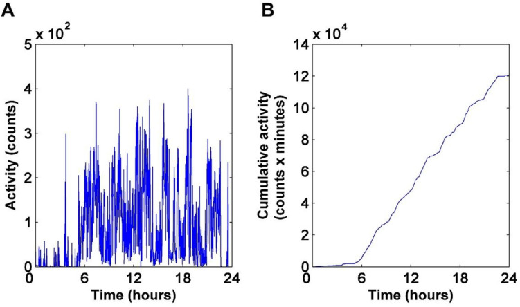
Human physical activity (HPA), a fundamental physiological signal characteristic of bodily motion is of rapidly growing interest in multidisciplinary research. Here we report the existence of hitherto unidentified hierarchical levels in the temporal organization of HPA on the ultradian scale: on the minute's scale, passive periods are followed by activity bursts of similar intensity ('quanta') that are organized into superstructures on the hours- and on the daily scale. The time course of HPA can be considered a stochastic, quasi-binary process, where quanta, assigned to task-oriented actions are organized into work packages on higher levels of hierarchy. In order to grasp the essence of this complex dynamic behaviour, we established a stochastic mathematical model which could reproduce the main statistical features of real activity time series. The results are expected to provide important data for developing novel behavioural models and advancing the diagnostics of neurological or psychiatric diseases.

Figure 1

(A) A typical daily activity recording taken by an actigraph. Acceleration values were recorded by 40 Hz sampling frequency, and the integration time was 1 min. for each depicted data point. (B) The running integral function (cumulative sum) of the time series in (A).

Figure 2

Probability density functions of activity spikes recorded under conditions described in Fig. 1. Curves in (A) and (B) are obtained from the original daytime activity recordings and the scrambled control, respectively. The time scale of the daily recordings was divided into equal intervals (“boxes”), and activity values were averaged within each box, respectively. PDF functions were calculated from these averaged values. Data are shown for some characteristic, quasi-exponentially distributed box lengths (1, 2, 5, 11, 22, 45, 90, 180, 360, and 720 min) distinguished by different colours (blue, green, red cyan, magenta, yellow, black, blue-green, red), respectively.

Figure 3

Log–log plots of probability density functions of the lengths of active and passive periods the original daytime recordings were divided into (orange and blue symbols, respectively). A period was considered active if its average activity was higher than 20 counts/min, and passive otherwise. Active PDFs were fitted by lognormal distributions defined by the conventional μ and σ parameters (μ_act = 3.5, σ_act = 1.3), while the linear decay of the passive PDF values in log–log representation clearly indicates a power-law function (slope ≈ − 2.67).

Figure 4

Multiscale representation of the daytime activity recordings. (A) Continuous wavelet decomposition of the motion activity signal corresponding to the concatenated wakeful periods of three subsequent days based on the Morlet wavelet. For a better visual demonstration, the wavelet coefficients were divided by $\sqrt{s}$, where $s$ is the scale parameter to ensure the scale-independent weight of the different patterns. Deep red and deep blue patches correspond to domains of maximal positive and minimal negative coefficients (1 and − 1, respectively), while green colour corresponds to values close to zero. (C) The result of the same wavelet decomposition if the individual data points within each period were randomly scrambled to remove temporal correlations. (B) Distribution of the square power of the wavelet coefficients over the scale dimension, calculated from the data of 10 subsequent days (blue: original, red: scrambled data). The three horizontal lines separate four well-distinct time-window ranges (Ranges 1–4, corresponding to intervals of ca. 1–20 min, 20 min–3 h, 3–10 h and > 10 h, respectively) of the most typical activity patterns, distinguished via the comparison of the two curves in (B). Inserts (D), (E) and (F), respectively, show the results of an analogous evaluation procedure of the corresponding sleep data comprising a concatenated nocturnal time series of 10 successive days. (D and F are the CW-maps of the original and scrambled data, while E shows the distribution of the square power of the wavelet-coefficients: blue: original, red: scrambled control).

Figure 5

Demonstration of the occurrence of elementary activity bursts by an integrate-and-fire electric-circuit model. (A) Capacitor (C) is charged by a constant current (I_t) superimposed to a Gaussian white noise of half-width δ, and a discharge takes place when the cumulative voltage on C (U_C) exceeds an upper threshold, taken as unity. (B) Simulated U_C voltage (blue line), and the corresponding burst events (grey bars). Please be aware that in panel (B), the scale of the positive y-axis has been magnified by a factor of 25 to enhance visibility.

Figure 6

PDF-analysis of the simulated time series (A), and the randomized control (B), in a log–log representation, analogous to Fig. 2. (C) Distribution of active (orange symbols) and passive (blue symbols) periods in a log–log representation analogous to Fig. 3. A period was considered active if its average amplitude for a 5-min time window exceeded 20 counts/min, and passive if the time window did not exceed the 20 counts/min.

Figure 7

Wavelet analysis of the simulated time-series data provided by the stochastic model in Fig. 5, with considering the “mid-day pause”, as a moderate modulation of the charge current, following Fig. S4. (A) The colour-coded continuous-wavelet maps of the simulated activity bursts are shown, (C) is the same for the randomized time series. (B) Shows the corresponding structuredness parameter as a function of the time window (i.e., the distribution of the square-power of the wavelet coefficients over the scale dimension).

References

1. Maczak B, Vadai G, Der A, Szendi I, Gingl Z. Detailed analysis and comparison of different activity metrics. PLoS One. 2021;16:e0261718. doi: 10.1371/journal.pone.0261718. - DOI - PMC - PubMed
1. Fekedulegn D, et al. Actigraphy-based assessment of sleep parameters. Ann. Work Expo Health. 2020;64:350–367. doi: 10.1093/annweh/wxaa007. - DOI - PMC - PubMed
1. Leuenberger, K. D. Long-Term Activity and Movement Monitoring in Neurological Patients (ETH Zürich, 2015).
1. Faedda GL, et al. Actigraph measures discriminate pediatric bipolar disorder from attention-deficit/hyperactivity disorder and typically developing controls. J. Child Psychol. Psychiatry. 2016;57:706–716. doi: 10.1111/jcpp.12520. - DOI - PMC - PubMed
1. Ancoli-Israel S, et al. The role of actigraphy in the study of sleep and circadian rhythms. Sleep. 2003;26:342–392. doi: 10.1093/sleep/26.3.342. - DOI - PubMed