End-to-end deep learning approach to mouse behavior classification from cortex-wide calcium imaging

Abstract

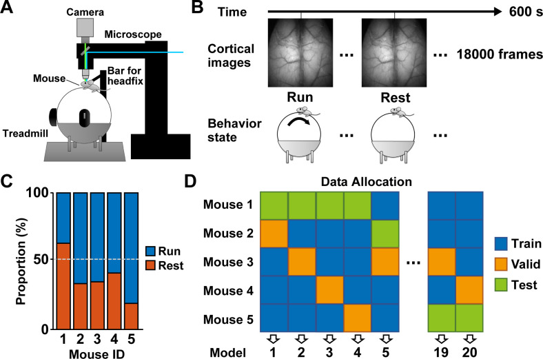
Deep learning is a powerful tool for neural decoding, broadly applied to systems neuroscience and clinical studies. Interpretable and transparent models that can explain neural decoding for intended behaviors are crucial to identifying essential features of deep learning decoders in brain activity. In this study, we examine the performance of deep learning to classify mouse behavioral states from mesoscopic cortex-wide calcium imaging data. Our convolutional neural network (CNN)-based end-to-end decoder combined with recurrent neural network (RNN) classifies the behavioral states with high accuracy and robustness to individual differences on temporal scales of sub-seconds. Using the CNN-RNN decoder, we identify that the forelimb and hindlimb areas in the somatosensory cortex significantly contribute to behavioral classification. Our findings imply that the end-to-end approach has the potential to be an interpretable deep learning method with unbiased visualization of critical brain regions.

Fig 1. Cortical activity and behavioral states in behaving mice.

(A) A schematic illustration of the experimental setup for measuring mesoscopic cortical calcium imaging and locomotor activity. (B) Images were obtained at 30 frames per second during a 600 s session. The label of behavioral state was based on locomotion speed (>0.5 cm/s) at the corresponding frame. (C) Proportions of the behavioral states in each mouse (n = 11–14 sessions from 5 mice). (D) The data allocation on a per-mouse basis. The data of each mouse was assigned at the ratio of 3:1:1 for training (Train), validation (Valid), and testing (Test).

Fig 2. Behavioral state classification using deep learning with CNN.

(A) Image preprocessing for deep learning with CNN. An image at frame t with images at neighboring frames (frame t −1 and t +1) was converted to an RGB image (image I_t) labeled with the behavioral state. (B) Schematic diagram of the CNN decoder. CNN was trained with individual RGB images. Then, CNN outputs the probability of running computing from the 1,280 extracted features for each image. (C) Schematic diagram of the CNN-RNN decoder. The pre-trained CNN extracted 1,280 features from individual RGB images in the first step. In the second step, a series of 1,280 extracted features obtained from consecutive images (e.g., eleven images from I_t −5 to I_t +5 (= input window, length ±0.17 s)) were input to GRU-based RNN. Then, the RNN output probability of running. (D) Loss of CNN and CNN-GRU during training and validation across three epochs. (E) The area under the receiver operating characteristic curves (AUC) was used to indicate the accuracy of decoders. The performance of decoders with CNN, CNN-LSTM, and CNN-GRU. ***P < 0.001, Wilcoxon rank-sum test with Holm correction, n = 20 models. (F) The performance of CNN-GRU decoders using smaller time windows gradually deteriorated while not above the 0.17 s lengths of the input window. **P < 0.01, N.S., not significant, Wilcoxon rank-sum test with Holm correction, n = 20 models.

Fig 3. Visualization of essential features in CNN-RNN decoder.

(A) An importance score was calculated by averaging differences from classification accuracy using a 1/16 masking area in each image (see Methods for details). (B) Importance scores in each subdivision (mean ± SD, n = 20 models). (C) Overlay of importance scores on the cortical image with ROI positions. See S2 Fig for ROIs 1–50.

Fig 4. Behavioral state classification from cortical activity using deep learning with RNN.

(A) Schematic overview of the RNN decoder for the behavioral state classification. Input is the cortical activities ranging from 0.5 s before (t−15 frames) to 0.5 s after (t+15 frames) the target frame t, which is labeled with a behavior state (1: run, 0: rest). The RNN decoder outputs the probability of behavioral states for all frames of testing data. (B–D) Example of the GRU decoder performance. (B) Learning curve during training and validation across 30 epochs. Loss indicates the cross entropy loss between the outputs and behavioral labels. Accuracy was the percentage of agreement with the label when the output was binarized at a 0.5 threshold. Mean ± SD, n = 20 models. (C) A trace of the output values of a representative decoder and actual behavioral labels in the first 33.3 s of testing data. (D) The receiver operating characteristic curves in the training, validation, and testing data. (E) The performance of GRU decoders trained with preprocessed data (GRU), non-preprocessed data (Raw), and the decoder of the linear regression model (LR). ***P < 0.001, Wilcoxon rank-sum test with Holm correction, n = 20 models. (F) The decoder performance using six types of RNN architectures. LSTM, GRU, simple RNN (Simple), and their bidirectional ones (Bi-). *P < 0.05, Wilcoxon rank-sum test with Holm correction, n = 20 models.

Fig 5. Comparison of input window length and target label’s temporal position.

(A) Examples of input window and position of the target labels for behavior classification were shown. “Length” defines the duration of the input window, which ranges arbitral time (e.g., 0.5 s) before and after the center of the input window (0 s). “Shift” defines the temporal location of the target label of behavior classification from the center of the input window. The length 0.5 s and the shift 0 s were used for the criteria for evaluation. (B) The decoder performance of different lengths using a fixed shift 0 s. *P < 0.05, **P < 0.01, Wilcoxon rank-sum test with Holm correction, n = 20 models. (C) The decoder performance of different shifts using a fixed length of 0.5 s. N.S., not significant, *P < 0.05, **P < 0.01, ***P < 0.001, Wilcoxon rank-sum test with Holm correction compared with shift 0 s, n = 20 models.

Fig 6. The forelimb and hindlimb areas of the somatosensory cortex contribute to behavioral state classification.

(A) The absolute SHAP values at each ROI during the input window across all GRU decoders (50 ROIs × 31 frames (−0.5 ~ 0.5 s) on 20 models average). (B) The absolute SHAP values for all frames at each ROI in GRU decoders with preprocessing data (GRU) and randomly shuffled data (Random). *P < 0.05, **P < 0.01, ***P < 0.001, Wilcoxon rank-sum test with Holm correction, n = 20 models. See S2 Fig for ROIs 1–50. (C) Red ovals indicate the position of the somatosensory cortex anterior forelimb and hindlimb areas (ROIs 6, 8, 31, and 33). (D) Decoder performance using fluorescent signals from all cortical areas (All), somatosensory cortex anterior forelimb and hindlimb areas (FLa&HLa, ROIs 6, 8, 31, and 33), and the other 46 ROIs (Other). ***P < 0.001, Wilcoxon rank-sum test with Holm correction, n = 20 models. (E) The ROIs were divided into five parts: motor areas (M2&M1, ROIs 1–4 and 26–29), somatosensory limb areas (FL&HL, ROIs 6–9 and 31–34), parietal and retrosplenial areas (PT&RS, ROIs 14–17 and 39–42), primary visual and visual medial areas (V1&Vm, ROIs 18–21 and 43–46), and visual lateral and auditory area (Vl&A1, ROIs 22–25 and 47–50). (F) Decoder performance using fluorescent signals from M2&M1, FL&HL, PT&RS, V1&Vm, and Vl&A1. ***P < 0.001, Wilcoxon rank-sum test with Holm correction, n = 20 models.

References

1. Craik A, He Y, Contreras-Vidal JL. Deep learning for electroencephalogram (EEG) classification tasks: a review. Journal of neural engineering. 2019. Apr 9;16(3):031001. doi: 10.1088/1741-2552/ab0ab5 - DOI - PubMed
1. LeCun Y, Bengio Y, Hinton G. Deep learning. nature. 2015. May 28;521(7553):436–44. - PubMed
1. Livezey JA, Glaser JI. Deep learning approaches for neural decoding across architectures and recording modalities. Briefings in bioinformatics. 2021. Mar;22(2):1577–91. doi: 10.1093/bib/bbaa355 - DOI - PubMed
1. Hochberg LR, Bacher D, Jarosiewicz B, Masse NY, Simeral JD, Vogel J, et al.. Reach and grasp by people with tetraplegia using a neurally controlled robotic arm. Nature. 2012. May 17;485(7398):372–5. doi: 10.1038/nature11076 - DOI - PMC - PubMed
1. Pan G, Li JJ, Qi Y, Yu H, Zhu JM, Zheng XX, et al.. Rapid decoding of hand gestures in electrocorticography using recurrent neural networks. Frontiers in neuroscience. 2018. Aug 27;12:555. doi: 10.3389/fnins.2018.00555 - DOI - PMC - PubMed