Classification of likely functional class for ligand binding sites identified from fragment screening

Abstract

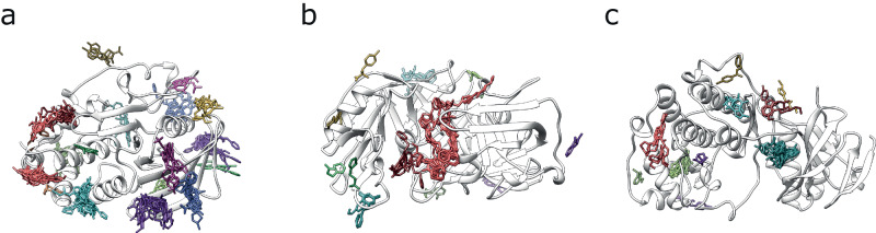
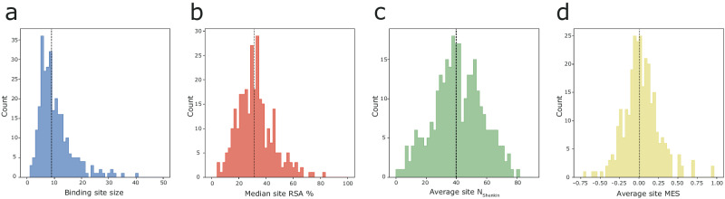
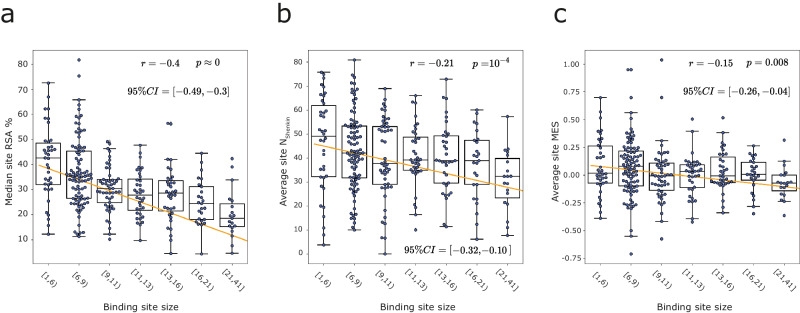
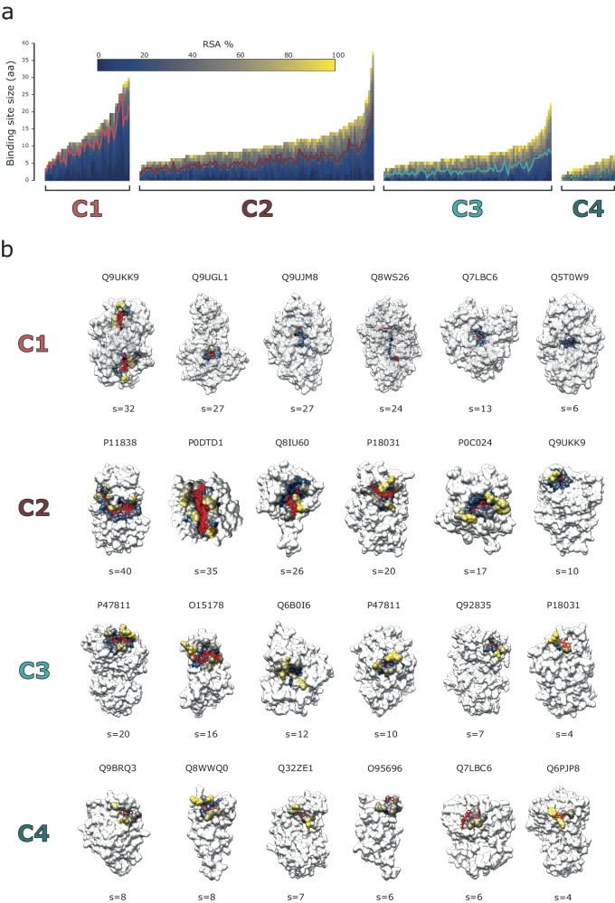
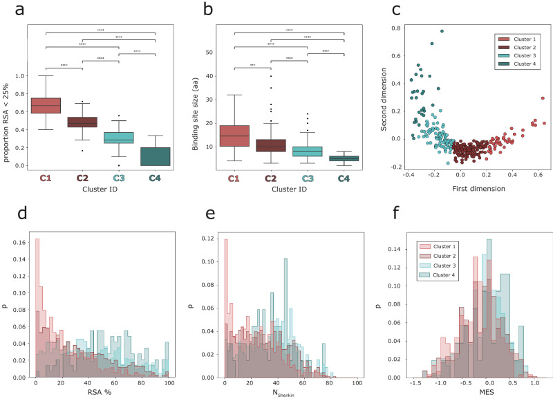
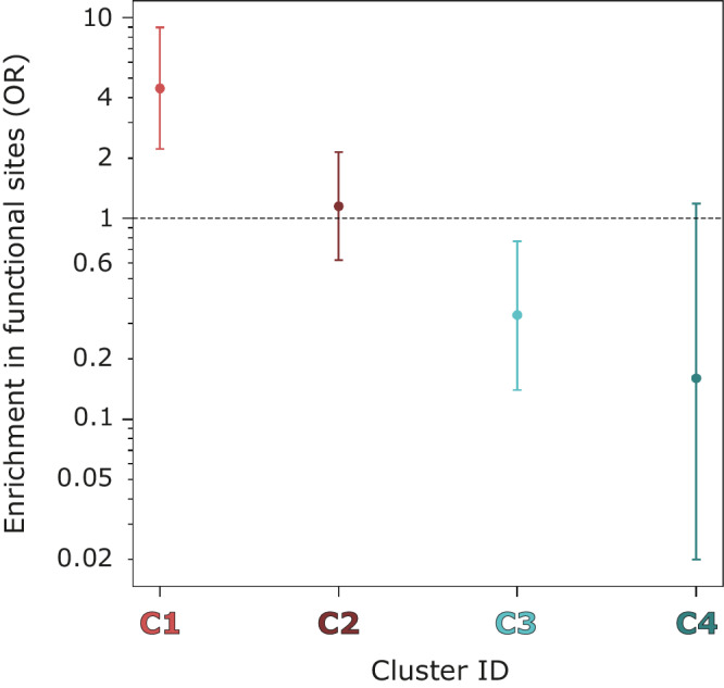
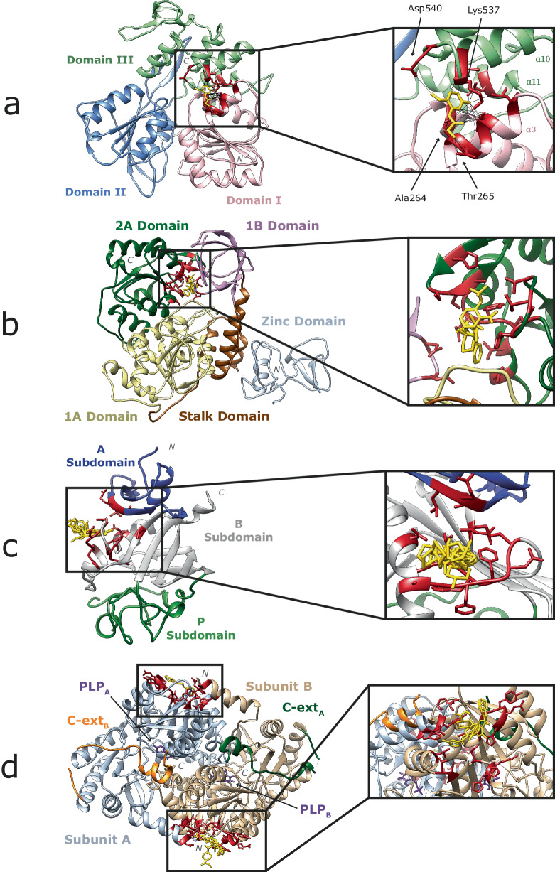
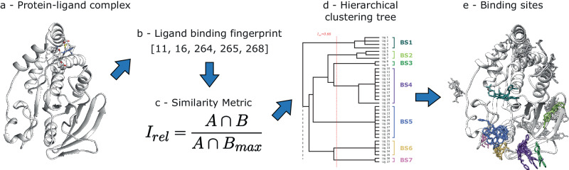
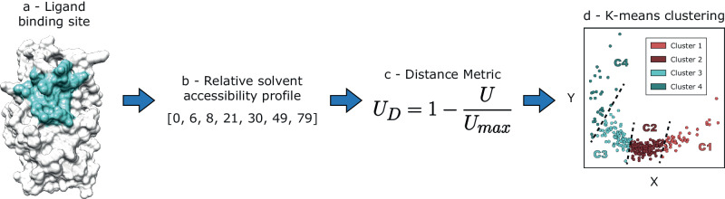
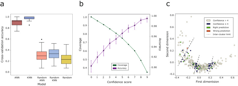
Fragment screening is used to identify binding sites and leads in drug discovery, but it is often unclear which binding sites are functionally important. Here, data from 37 experiments, and 1309 protein structures binding to 1601 ligands were analysed. A method to group ligands by binding sites is introduced and sites clustered according to profiles of relative solvent accessibility. This identified 293 unique ligand binding sites, grouped into four clusters (C1-4). C1 includes larger, buried, conserved, and population missense-depleted sites, enriched in known functional sites. C4 comprises smaller, accessible, divergent, missense-enriched sites, depleted in functional sites. A site in C1 is 28 times more likely to be functional than one in C4. Seventeen sites, which to the best of our knowledge are novel, in 13 proteins are identified as likely to be functionally important with examples from human tenascin and 5-aminolevulinate synthase highlighted. A multi-layer perceptron, and K-nearest neighbours model are presented to predict cluster labels for ligand binding sites with an accuracy of 96% and 100%, respectively, so allowing functional classification of sites for proteins not in this set. Our findings will be of interest to those studying protein-ligand interactions and developing new drugs or function modulators.

Fig. 1. Ligand clusters defined by the binding site definition algorithm.

For simplicity, only one protein chain ribbon is shown in white for each example. Ligands are coloured according to the site they bind to. Identifiers are from UniProt. a There were 110 structures depicting human tyrosine-protein phosphatase non-receptor type 1 (PTPN1), P18031, binding 143 ligand molecules, 104 of which were unique. 18 binding sites were defined. b The 68 ligands, 30 unique, found across 50 structures of the chestnut blight fungus endothiapepsin (EAPA), P11838, were classified in 12 distinct binding sites. c For mouse mitogen-activated protein kinase 14 (Mapk14), P47811, 52 structures portrayed the interaction with 53 ligand molecules, 50 unique, which clustered in 10 ligand binding sites.

Fig. 2. Variation in binding site features.

Distribution of a size, b median RSA, c N_Shenkin and d MES across the 293 binding sites defined from our dataset. Black dashed lines indicate the median of each distribution.

Fig. 3. Relation between different binding site properties.

A regression line is fitted to all data points previous to binning, (N = 293 binding sites), Pearson’s correlation coefficient r, associated p-value and 95% CI of r. Data points are grouped into bins according to different binding site size intervals, represented by box and swarm plots. a Median site RSA % vs binding site size, in amino acids. b Average N_Shenkin vs binding site size. c Average site MES vs site size. Boxes represent the IQR, and whiskers extend to $1.5\times \mathrm{IQR}$.

Fig. 4. RSA-based binding site clusters and examples.

a RSA profiles of the 293 binding sites that were grouped in four, C1-C4, clusters by K-means based on the difference between their RSA profiles (U_D). Each binding site is represented by a vector, plotted as a bar here. The elements of the vector represent the residues that form the binding site and are sorted according to their RSA, so buried residues are at the beginning of the vector (bottom), and more accessible residues towards the end (top). Each element of the vector, or section of the bar, is coloured according to RSA, using the matplotlib cividis colour palette. Within each cluster, binding sites are sorted based on the number of amino acids. Over each cluster, a line is drawn at RSA = 25%. b Six examples of binding sites are shown in structure for each cluster. Examples were selected to represent the range of binding site sizes within each cluster. IDs are UniProt accession codes. Binding site residues are coloured according to their RSA, using the cividis colour scheme. The rest of the protein is coloured in white. Ligands binding to the site in question are coloured in red.

Fig. 5. Binding site cluster features.

a Box plot of the proportion of residues with RSA < 25% per binding site across the four clusters defined by K-means clustering. b Box plot of the binding site size, in amino acids, across clusters. Pairwise Mann–Whitney–Wilcoxon tests were performed to assess the differences between the clusters. Boxes represent the IQR, and whiskers extend to $1.5\times \mathrm{IQR}$. p-value annotation legend: $ns:p>0.05$, $*:0.01<p\le 0.05$, $**:{10}^{-2}<p\le {10}^{-3}$, $***:{10}^{-4}<p\le {10}^{-3}$, $****:p\le {10}^{-4}$. c MDS representation of the 293 binding sites on 2 dimensions. Data points represent binding sites and are coloured based on the cluster they group in. d Histogram of RSA % of the residues found within the ligand binding sites in each cluster. e Histogram of N_Shenkin within cluster residues. f MES histogram plots for the four clusters defined.

Fig. 6. Binding site cluster enrichment in known functional sites.

This enrichment score is an odds ratio (OR). Error bars indicate 95% CI of the OR. Y axis is in log₁₀ scale. A pseudo-count of 1 was added to each cell of the contingency table to calculate the score.

Fig. 7. Examples of C1 sites of interest.

a Non-structural protein NS3 of Zika virus (Q32ZE1) binding to N-(2-methoxy-5-methylphenyl)glycinamide, NY7 in BS7 (PDB: 5RHG) (Godoy AS, Mesquita NCMR, Oliva G). Domains I, II, and III are coloured in pink, blue, and green, respectively. Binding site 7 which is in Cluster 1 is highlighted, the other 9 binding sites which fall in C2 (3), C3 (3) and C4 (3) are hidden. Ligand binding residues in red, and NY7 in yellow. Protein–ligand interactions are represented by black lines. b Non-structural protein NSP13 of SARS-CoV-2 (P0DTD1) binding to three ligands in BS6 + 16 (Ribbon PDB: 5RMH). 1A, 1B, 2A, stalk and zinc domains are coloured in yellow, pink, green, brown, and grey, respectively. Ligand binding residues in red, and ligands in yellow. Interactions are not shown here for simplicity. c Human tenascin, TN, (P24821) binding to 8 ligands in BS0. (Ribbon PDB: 5R60) (Coker JA, Bezerra GA, von Delft F, Arrowsmith CH, Bountra C, Edwards AM, Yue WW, Marsden BD). A, B, and P subdomains as defined by Yee et al. are coloured in blue, grey, and green, respectively. d Human erythroid-specific mitochondrial 5-aminolevulinate synthase, ALAS-E, (P22557) binding to 7 ligands in BS1. (Ribbon PDB: 5QR0) (Bezerra GA, Foster W, Bailey H, Shrestha L, Krojer T, Talon R, Brandao-Neto J, Douangamath A, Nicola BB, von Delft F, Arrowsmith CH, Edwards A, Bountra C, Brennan PE, Yue WW). Subunits A, B, C-terminal extensions A, B, as well as PLP cofactors are coloured in grey, beige, green, orange, and purple, respectively. Ligand binding residues in red, and ligands in yellow.

Fig. 8. Ligand binding site definition algorithm.

The method defines ligand binding sites from a set of three-dimensional structures portraying the complex of a protein of interest bound to ligands. a Protein–ligand complex (P18031). b Ligand binding fingerprint, comprised by protein residue numbers interacting with ligand. c Formula of the similarity metric: relative intersection, I_rel. d Hierarchical clustering tree resulting from the similarity matrix, cut at threshold to determine distinct clusters of ligands. e Three-dimensional structure of all ligands binding to protein, coloured according to the cluster they group into. Only ligands found clusters 1–7 are in coloured based on their cluster membership. The rest are coloured in grey. The tree on (d) represents only a part of the tree, showing 7/18 binding sites defined on P18031. This is represented by a dash line pointing downwards on the tree.

Fig. 9. Binding site clustering algorithm.

The method here clusters ligand binding sites defined across different proteins based on their solvent accessibility profiles. a Example of a defined ligand binding site. b Relative solvent accessibility profile of a binding site, represented by the RSA of the site residues. c Formula of our distance metric: distance U, U_D. d Multidimensional scaling (MDS) representation of binding sites coloured according to the four clusters determined by the K-means algorithm. Dashed lines represent the cluster limits.

Fig. 10. MLP cross-validation and blind test results.

a Average accuracy of the 10-repeat 10-fold (N = 100) cross-validation of the KNN, and ANN predictive models compared to a baseline of the same models trained on randomly shuffled data, as well as complete random prediction $\left(p=0.25\right)$. The box represents the central 50% of the data, i.e., Q1 — median (Q2) — Q3, also known as interquartile range (IQR). Whiskers extend to 1.5 × IQR, and beyond them are the outliers. b Cross-validation accuracy and proportion of binding sites against cumulative confidence score from the trained ANN. Sites presenting a confidence score greater or equal to 5, the average accuracy is 97%, and the percentage of sites with this score is 75%. Predictions are for the 2660 cross-validation data points, 10 different repeats of 10 distinct splits of 26–27 binding sites each. Accuracy error bars indicate 95% CI of the proportion. c MDS representation of the 293 binding sites. Training data are coloured according to the average confidence of their prediction in the cross-validation. Test data are coloured according to whether they were correctly predicted or not. Dashed lines indicate the limits of K-means clusters.

References

1. Murray CW, Rees DC. The rise of fragment-based drug discovery. Nat. Chem. 2009;1:187–192. doi: 10.1038/nchem.217. - DOI - PubMed
1. Congreve M, et al. A ‘rule of three’ for fragment-based lead discovery? Drug Discov. Today. 2003;8:876–877. doi: 10.1016/S1359-6446(03)02831-9. - DOI - PubMed
1. Rees DC, et al. Fragment-based lead discovery. Nat. Rev. Drug Discov. 2004;3:660–672. doi: 10.1038/nrd1467. - DOI - PubMed
1. Schiebel J, et al. Six biophysical screening methods miss a large proportion of crystallographically discovered fragment hits: a case study. ACS Chem. Biol. 2016;11:1693–1701. doi: 10.1021/acschembio.5b01034. - DOI - PubMed
1. Krivak R, Hoksza D. P2Rank: machine learning based tool for rapid and accurate prediction of ligand binding sites from protein structure. J. Cheminform. 2018;10:39. doi: 10.1186/s13321-018-0285-8. - DOI - PMC - PubMed
Publication types