East Asian summer monsoon delivers large abundances of very-short-lived organic chlorine substances to the lower stratosphere

Abstract

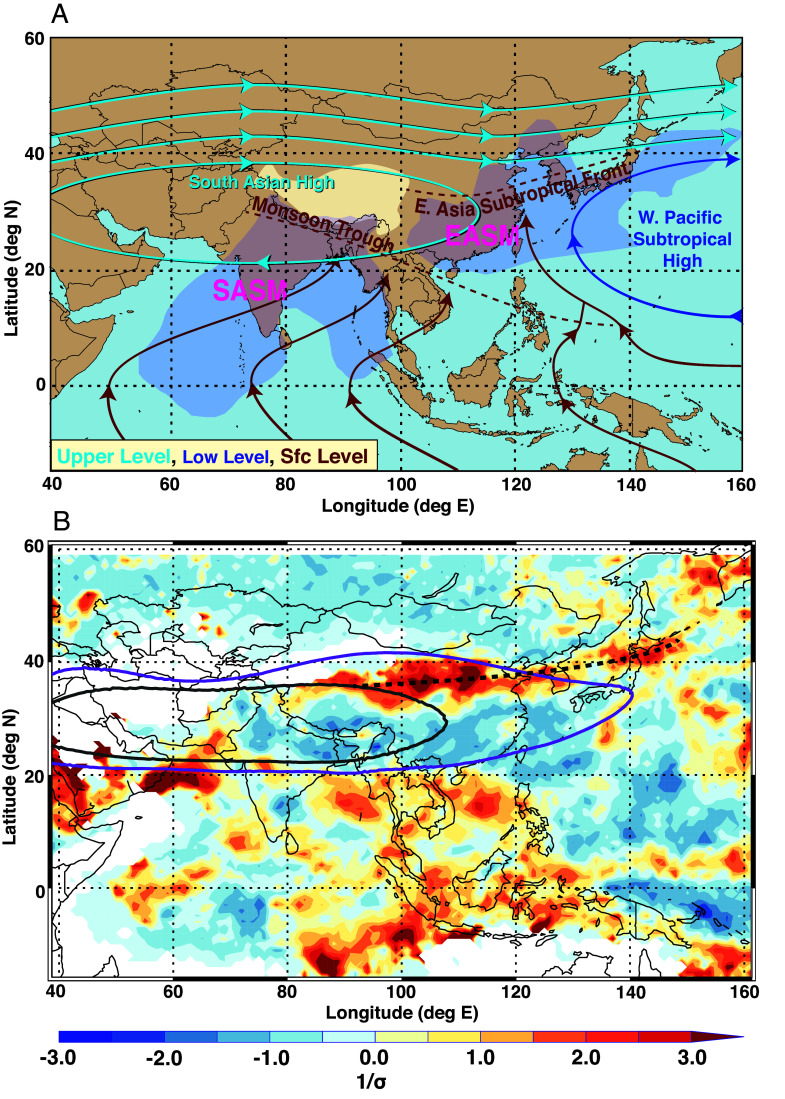
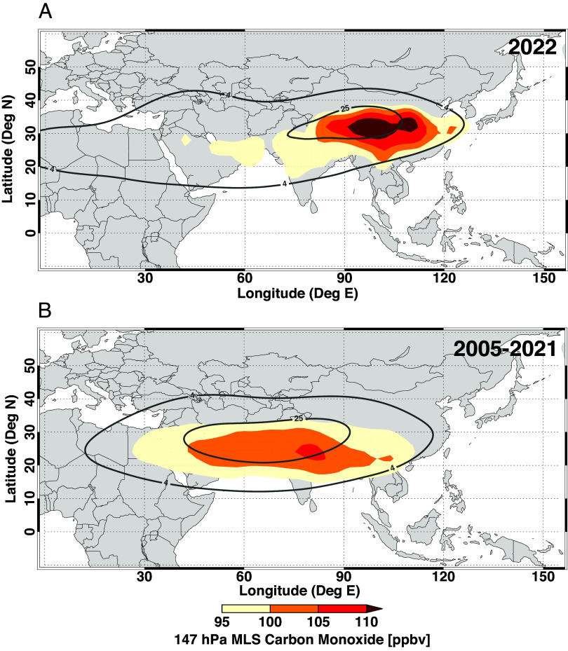
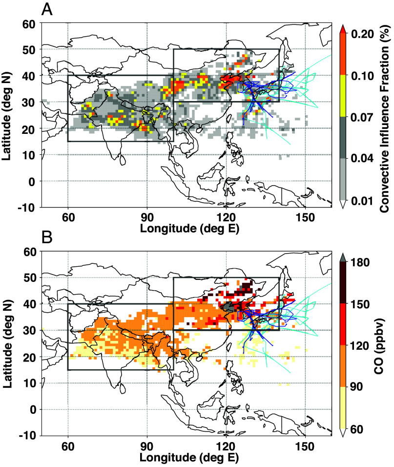
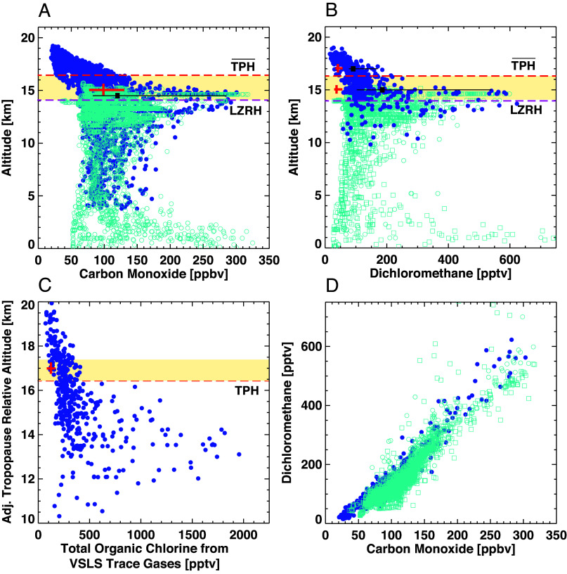
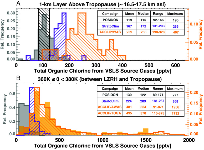
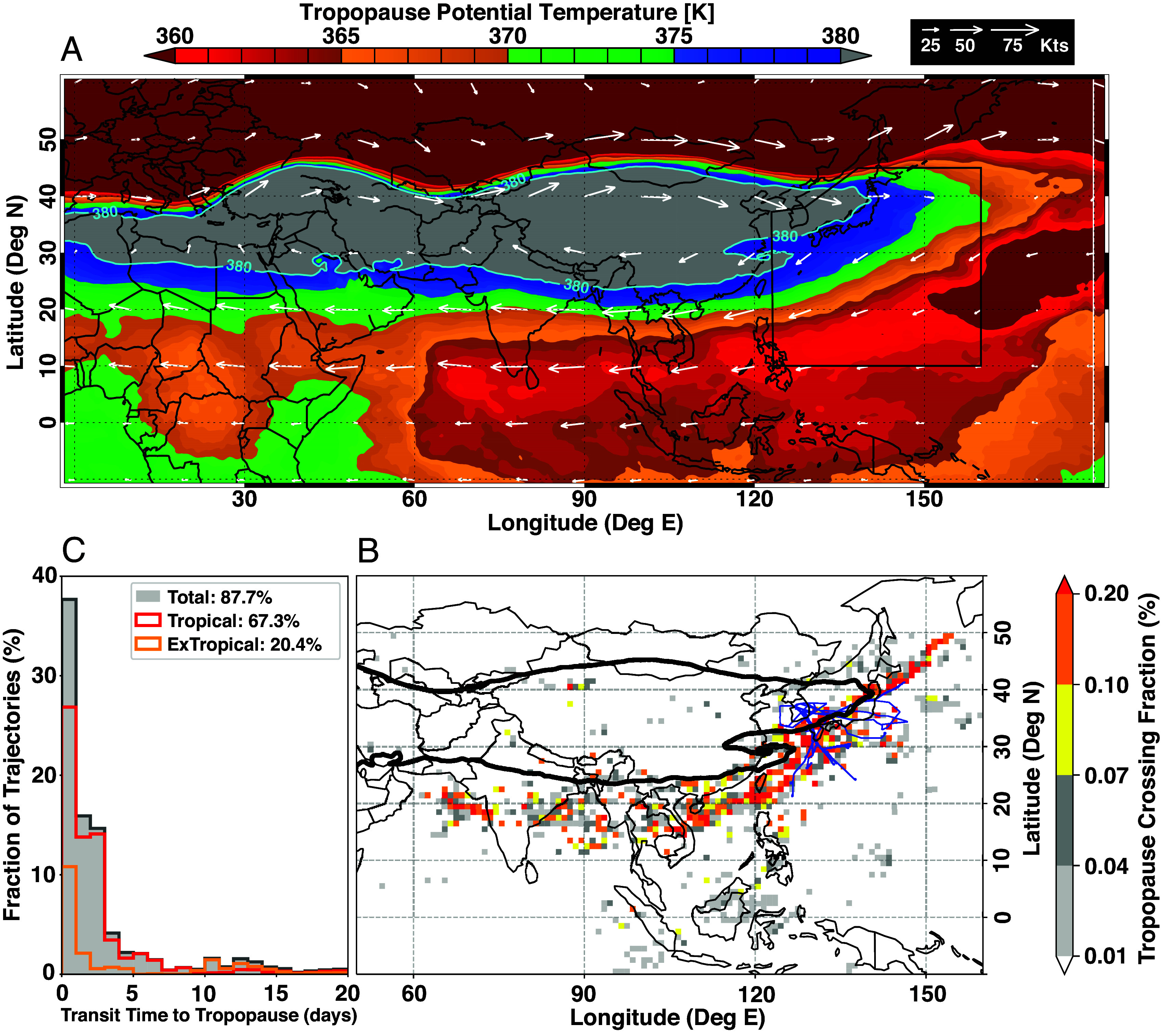
Deep convection in the Asian summer monsoon is a significant transport process for lifting pollutants from the planetary boundary layer to the tropopause level. This process enables efficient injection into the stratosphere of reactive species such as chlorinated very-short-lived substances (Cl-VSLSs) that deplete ozone. Past studies of convective transport associated with the Asian summer monsoon have focused mostly on the south Asian summer monsoon. Airborne observations reported in this work identify the East Asian summer monsoon convection as an effective transport pathway that carried record-breaking levels of ozone-depleting Cl-VSLSs (mean organic chlorine from these VSLSs ~500 ppt) to the base of the stratosphere. These unique observations show total organic chlorine from VSLSs in the lower stratosphere over the Asian monsoon tropopause to be more than twice that previously reported over the tropical tropopause. Considering the recently observed increase in Cl-VSLS emissions and the ongoing strengthening of the East Asian summer monsoon under global warming, our results highlight that a reevaluation of the contribution of Cl-VSLS injection via the Asian monsoon to the total stratospheric chlorine budget is warranted.

Keywords: Asian summer monsoon; convective transport; stratospheric ozone; very-short-lived ozone-depleting substances.

Fig. 1.

ASM subcomponents and the active East Asian monsoon in August 2022. (A) Schematic of Asian summer monsoon subcomponents (14, 15). Flow patterns are shown at three levels represented by near surface (1,000 hPa “Sfc Level”), low level (850 hPa), and upper level (200 hPa). The East Asia Subtropical Front is the major rainfall-producing system; it is located on the northwest flank of the Western Pacific Subtropical High and migrates seasonally from around 25°N in May to 40°N in August. From mid-June to mid-July, the front is generally located from the Yangtze River basin to southern Japan, and the corresponding rainy season is called Meiyu in China or Baiu in Japan (16). (B) August 2022 anomalies of the occurrence frequency of convection defined by infrared brightness temperature T_B < 235 K using GPM MERGIR satellite data (17). The criterion identifies convective cloud tops above ~12 km altitude. Anomalies are calculated with respect to the climatological (2006–2022) August mean occurrence frequency at each location and scaled by the SD (σ). The position of the East Asia Subtropical Front for August 2022 is highlighted (black dashed curve). Also shown are 150 hPa geopotential height from the NCEP Climate Forecast System (CFS) data (18) 14,350-m contours for the 44-y (1979–2022) August climatology (gray) and August 2022 (purple)

Fig. 2.

Chemical signature of the strong EASM convective transport in 2022 from space. August average upper tropospheric carbon monoxide (CO) mixing ratios from satellite retrievals (MLS version 5 data at 147 hPa; see ref. for details of MLS data quality and resolution) for (A) 2022 and (B) 2005–2021. Also shown are two selected contours of the 150 hPa stream function ([4, 25] × 10⁶ m²/s; based on the NCEP CFS data), which mark the outer edge and the center location of the ASM anticyclone.

Fig. 3.

Airborne observations of convective transport from SASM and EASM. (A) ACCLIP airborne campaign flight tracks (July 31 to September 1, 2022) and trajectory model derived convective influence (Materials and Methods). The distribution of convective influence for the airborne measurements at high altitudes (<200 hPa), estimated using trajectory calculations to connect the flight tracks with convection. Shaded pixels (1 × 1 degree) show the relative frequency of the colocation between convective clouds and back trajectories from the flight tracks (Materials and Methods). (B) The distribution of average CO mixing ratios for all airborne samples with convective influence within each pixel. The average CO for samples connected to the SASM and EASM domains (gray boxes) are approximately 95 and 130 ppbv, respectively. Note that the SASM average is consistent with the StratoClim measurements (33, 34). The blue and cyan lines show the flight tracks for the two research aircraft: the NASA WB-57 and the NSF/NCAR GV, respectively.

Fig. 4.

Record-breaking CO and Cl-VSLS observed in the UTLS. (A) Vertical distribution of CO mixing ratios measured on the WB-57 (blue) and GV (cyan) aircraft (Materials and Methods) from all research flights (July 31 to September 1, 2022). The mean value and the 5th to 95th percentile for the 1-km layer near the level of zero clear-sky radiative heating (LZRH, magenta dashed line), approximated here by 360 K potential temperature (35), are marked by the filled black square and the thin black line, respectively. The average tropopause height is 16.5 km or ~380 K (red dashed line labeled TPH). The layer between the LZRH and the average tropopause is shaded in beige. The mean and range, represented by the 5th and 95th percentiles, for the StratoClim CO data (33) at the same levels are marked by the red vertical and horizontal lines, respectively. (B) Same as A but for dichloromethane (CH₂Cl₂) measured by WAS on WB-57 and TOGA and AWAS from the GV (Materials and Methods). For reference, the red symbols show the mean and range from previous measurements from the tropical tropopause region (see Tables 1-5 in ref. 19) and for the tropopause layer, 16.5 to 17.5 km. (C) Vertical distribution of total chlorine from WB-57 WAS measurements (Materials and Methods) of five primary Cl-VSLSs in tropopause-relative coordinates, adjusted by the mean tropopause height of 16.5 km (ref. their equation 1). The red symbol marks the mean and range from previous measurements (see tables 1-5 in ref. 19). (D) A general positive correlation between CH₂Cl₂ and CO exemplifies the strong correlation between CO and many PBL pollutants measured during ACCLIP.

Fig. 5.

Total VSLS-sourced organic chlorine. The relative frequency distributions of total organic chlorine from five Cl-VSLS source gases (dichloromethane, chloroform, 1,2-dichloroethane, 1,2-dichloropropane, and tetrachloroethene) from ACCLIP measurements (orange, right-hand y axis) in two layers: (A) within 1 km above the tropopause, representing the lower stratosphere (LS), and (B) 360 to 380 K potential temperature, representing the upper troposphere (UT) between the LZRH and the tropopause. The ACCLIP UT data in B were obtained by two instruments: TOGA-TOF (shaded) and AWAS/WAS (striped) (Materials and Methods). The LS data in A are from the WB-57 WAS measurements (Materials and Methods). Also shown for comparison in both (A) and (B) are WAS measurements over the tropical western Pacific during the October 2016 POSIDON campaign (gray; note that 1,2-dichloropropane was not included) and WAS measurements mostly sampling the SASM contribution during the summer 2017 StratoClim campaign (purple, sharing gray axis with POSIDON; note that 1,2-dichloropropane and tetrachloroethene were not included). The estimated contribution of Cl-VSLS source gases to the stratospheric chlorine budget in 2020 used in the 2022 WMO Ozone Assessment (105 ± 20 ppt) is shown in A (black). Mean, median, range (mean ± 1 σ), and maximum values of the total Cl-VSLSs for each dataset are given in the insets. Note that in (A) the POSIDON samples (106 cans) are selected within the 16.5 to 17.5 km layer, whereas the ACCLIP LS samples (69 cans) are selected within 1 km above the tropopause as determined using the nearest WB-57 in situ measurements. StratoClim samples (29 cans) are selected within 1 km above the tropopause using the ERA5 tropopause product (43).

Fig. 6.

August 2022 tropopause structure in potential temperature and the trajectory model diagnosis of the UT air mass entering the stratosphere. (A) The August 2022 monthly mean tropopause in potential temperature (color shaded contours) based on the ERA5 tropopause product (43). Also shown are the ERA5 horizontal winds at the 380 K level (white overlaid arrows). The rectangle (black) indicates the nominal ACCLIP flight region (Fig. 3). (B) The relative frequency map of the air mass tropopause crossing locations for all WB-57 WAS samples in the UT layer (between 360 K and the tropopause) (Materials and Methods). The WAS sampling locations are distributed along the WB-57 flight tracks (blue lines). To highlight the relationship between tropopause crossing frequency and the tropopause structure associated with the ASM anticyclone shown in panel A, the August 2022 monthly mean tropopause potential temperature at 380 K is shown (black contour). (C) Histogram of the fractions of trajectories crossing the tropopause within 20 d and their transit time distributions: the total fraction of sampled air masses that crossed the tropopause (gray), the fraction that followed the anticyclonic flow and entered the tropical lower stratosphere (red), and the fraction that entered the mid- to high-latitude lowermost stratosphere (orange). The tropical/extratropical separation is approximated by whether a trajectory’s tropopause intercept was south or north (respectively) of the WAS measurement point at which a given trajectory was initialized.

References

1. Randel W. J., et al. , Asian monsoon transport of pollution to the stratosphere. Science 328, 611–613 (2010), 10.1126/science.1182274. - DOI - PubMed
1. Park M., Randel W. J., Gettelman A., Massie S. T., J. H., Jiang Transport above the Asian summer monsoon anticyclone inferred from Aura Microwave Limb Sounder tracers. J. Geophys. Res. 112, D16309 (2007), 10.1029/2006JD008294 - DOI
1. Vernier J.-P., Thomason L. W., Kar J., CALIPSO detection of an Asian Tropopause Aerosol Layer. Geophys. Res. Lett. 38, L07804 (2011), 10.1029/2010GL046614. - DOI
1. Santee M. L., et al. , A comprehensive overview of the climatological composition of the Asian summer monsoon anticyclone based on 10 years of Aura Microwave Limb Sounder measurements. J. Geophys. Res. Atmos. 122, 5491–5514 (2017), 10.1002/2016JD026408. - DOI
1. Yu P., et al. , Efficient transport of tropospheric aerosol into the stratosphere via the Asian summer monsoon anticyclone. Proc. Natl. Acad. Sci. U.S.A. 114, 6972–6977 (2017), 10.1073/pnas.17011701. - DOI - PMC - PubMed
LinkOut - more resources