Imaging and Molecular Annotation of Xenographs and Tumours (IMAXT): High throughput data and analysis infrastructure

Abstract

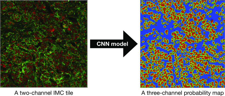
With the aim of producing a 3D representation of tumors, imaging and molecular annotation of xenografts and tumors (IMAXT) uses a large variety of modalities in order to acquire tumor samples and produce a map of every cell in the tumor and its host environment. With the large volume and variety of data produced in the project, we developed automatic data workflows and analysis pipelines. We introduce a research methodology where scientists connect to a cloud environment to perform analysis close to where data are located, instead of bringing data to their local computers. Here, we present the data and analysis infrastructure, discuss the unique computational challenges and describe the analysis chains developed and deployed to generate molecularly annotated tumor models. Registration is achieved by use of a novel technique involving spherical fiducial marks that are visible in all imaging modalities used within IMAXT. The automatic pipelines are highly optimized and allow to obtain processed datasets several times quicker than current solutions narrowing the gap between data acquisition and scientific exploitation.

Keywords: Data management; data processing and analysis; fluorescence microscopy; imaging mass cytometry.

Figure 1.

IMAXT pipeline. Once a tumor has been extracted it is embedded in an agarose cube together with spherical beads. The sample is then analyzed in the STPT instrument where it is imaged and cut into thin slices and a multichannel 3D data cube is produced. The slices are then imaged with an Axioscan fluorescence microscope and an IMC mass cytometer. The spherical beads are used for alignment of slices within each sample and for registration between all samples. All imaging is resampled to the STPT reference. All data, including sequencing, is then federated to build an annotated 3D model.

Figure 2.

3D visualizations of two stitched STPT cubes with different properties. (a) Volumetric reconstruction from 99 sections of 15 μm This sample was processed by an orthotopic injection of the fluorescent 4 t1-E subclone⁽¹¹⁾ shown in channel 3 (green) which is known to undergo vascular mimicry. In addition, this sample was perfused with the DiI lipophilic dye seen in channel 2 (red) to highlight vessel structures. (b) Volumetric reconstruction from 100 sections of 25 μm, each with 5 optical sections of 5 μm from a 4 T1 tumor in a BalbC mouse with the tdTomato marker. The fluorescence beads are clearly visible in the medium outside the biological tissue and prove to be crucial for all stages of registration.

Figure 3.

Multi-modality image registration. Registration across different modalities is achieved using the spherical fiducial beads. These are automatically detected on single-channel images, and a measurement of their geometric center is obtained. The top row of images shows the location of detected beads in an Axioscan, STPT, and IMC slide. A first coarse alignment is carried out using 32× downsampled images, and with this and the fiducial center coordinates, an affine transformation matrix is calculated. With this, we can reproject between modalities. The result can be seen in the bottom panel, an inset of the box outlined in the STPT image once registration has finished; here Axioscan occupies the red channel, IMC the green, and STPT the blue.

Figure 4.

Analysis of IMC data segmentation of the 3D sample. (a) Marker abundance plots for a representative 2D section of the sample. Each dot is a segmented cells and signal intensity corresponds to the normalized abundance of the marker in the cell. We show GFP and TdTomato (tumor cell populations), proliferation (Ki67), and Hypoxia markers (Car9). (b) UMAP dimensional reduction plot for the dataset. (c) Spatial plot of a representative 2D section of the dataset. Each color corresponds to a different cell type predicted by leiden clustering on the data.

Figure 5.

Processing pipeline steps applied to both STPT and Axioscan raw image data. Note that in the experimental flow the STPT acquires the images of the slides and does the sectioning after which they are acquired with Axioscan.

Figure 6.

Average intensity per pixel. Normalized intensity averaged over columns ( , blue) and rows ( , orange) over the first tenth of the detector. The effect of background illumination is evident here. The first pixels are already truncated by the microscope software to eliminate the most contaminated areas.

Figure 7.

STPT flatfield correction. Left: Relative difference of overlapping pixels before (blue) and after (orange) flatfield correction. Right: Example of normalized flatfield frame.

Figure 8.

Effects of the distortion correction as applied to STPT tiles. Both panels show the same patch (500 px across in the Y direction) of two overlapping tiles. The ellipses highlight areas where distortion effects are most visible. Top: Distortion-corrected overlap. Bottom: Uncorrected overlap.

Figure 9.

STPT geometric distortion correction. Field of view optical distortion for STPT produced by the optics of the microscope. Maximum distortion in the corners of the image is of the order of 20 μm. This is corrected before the registration between tiles by resampling the images to an undistorted pixel space.

Figure 10.

Example final stitched STPT stage mosaic (left) with associated confidence map (right). Images are padded so that all slices from a sample have the same size, hence explaining the pixels with zero confidence at the right and lower ends of the confidence map.

Figure 11.

Histogram of projected radius of a sample of randomly selected beads. The projected radius is the apparent radius of a bead in an slice image.

Figure 12.

Example of the bead detection and profiling for an STPT mosaic. Panel (a) contains the original STPT image, (b) depicts the bead detection mask produced by the U-Net network, and (c) depicts the original image plus the fitted radius for each detected bead.

Figure 13.

Examples of the profiling function applied to measured STPT beads.

Figure 14.

Evolution of with slice number (i.e., depth along the sample). Dashed lines mark the error boundary. As can be seen, there is a drift in one of the directions, likely to be related to the effect of the microtome blade pushing into the sample cube. The scale for this sample is 0.56 μm per pixel.

Figure 15.

Top panel: Error in the recovered center coordinates for beads simulated at different S/N, as a fraction of the bead radius. The orange line represents a running median. At the median error reaches the asymptotic value denoted by the horizontal red line. Bottom panel: histogram of the measured S/N for a random sample of beads.

Figure 16.

Registration error as a function of the average number of beads on each slice. The high S/N regime corresponds to , while low S/N stands for .

Figure 17.

Dice-XMBD CNN model is used to convert a sample two-channel IMC tile (left) into a probability map (right). In both panels, red color is associated with nuclear marker and green represents the cytoplasm. The size of each tile is .

Figure 18.

A probability map (left panel) is split into 3-channels associated with background, nuclear, and cytoplasmic channels (middle panel). The outcome of the segmentation of probability map is cells/nuclei masks (right panel). The size of each tile is .

Figure 19.

Number of common beads between an Axioscan and all the STPT slices taken from the parent sample cube. The red line is the best Gaussian fit to the evolution of with , and the vertical line marks the predicted for .

Figure 20.

Axioscan to STPT slide matching algorithm.

Figure 21.

Cumulative distribution for the registration errors as measured through the reprojected center coordinates.

References

1. Ragan T, Kadiri LR, Venkataraju KU, et al. (2012) Serial two-photon tomography for automated ex vivo mouse brain imaging. Nat Methods 9(3), 255–258. - PMC - PubMed
1. Giesen C, Wang HAO, Schapiro D, et al. (2014) Highly multiplexed imaging of tumor tissues with subcellular resolution by mass cytometry. Nat Methods 11(4), 417–422. - PubMed
1. Alon S, Goodwin DR, Sinha A, et al. (2021) Expansion sequencing: spatially precise in situ transcriptomics in intact biological systems. Science 371, eaax2656. 10.1126/science.aax2656. - DOI - PMC - PubMed
1. Moffitt JR & Zhuang X (2016) RNA imaging with multiplexed error-robust fluorescence in situ hybridization (MERFISH). Methods Enzymol 572, 1–49. - PMC - PubMed
1. Walton NA, Brenton JD, Caldas C, et al. (2010) PathGrid: a service-orientated architecture for microscopy image analysis. Philos Trans A Math Phys Eng Sci 368(1925), 3937–3952. 10.1098/rsta.2010.0158. - DOI - PubMed
LinkOut - more resources