Histology-guided mathematical model of tumor oxygenation: sensitivity analysis of physical and computational parameters

Abstract

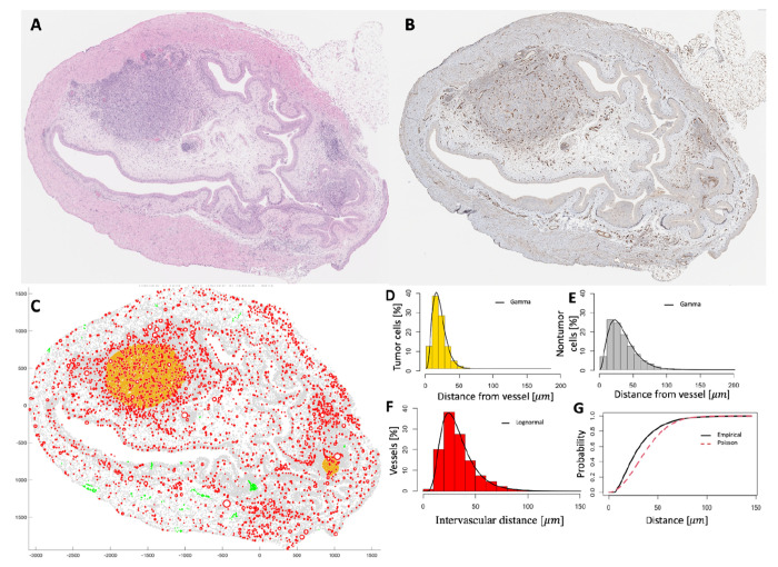
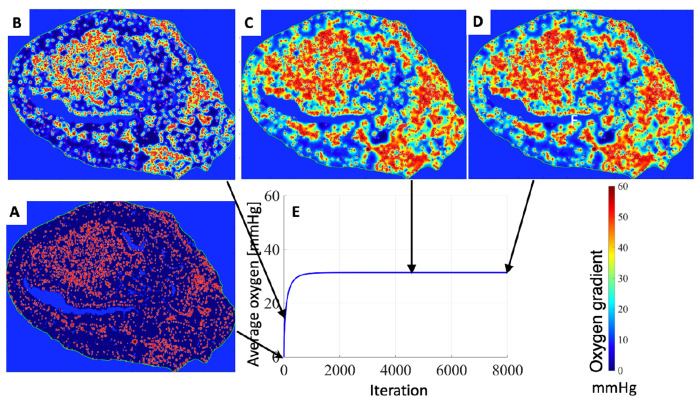
A hybrid off-lattice agent-based model has been developed to reconstruct the tumor tissue oxygenation landscape based on histology images and simulated interactions between vasculature and cells with microenvironment metabolites. Here, we performed a robustness sensitivity analysis of that model's physical and computational parameters. We found that changes in the domain boundary conditions, the initial conditions, and the Michaelis constant are negligible and, thus, do not affect the model outputs. The model is also not sensitive to small perturbations of the vascular influx or the maximum consumption rate of oxygen. However, the model is sensitive to large perturbations of these parameters and changes in the tissue boundary condition, emphasizing an imperative aim to measure these parameters experimentally.

Fig. 1.. Histology data and the digitized tissue.

A. A hematoxylin and eosin histology image of the tissue. The nuclei of tumor and nontumor cells are stained in deep blue-purple, and the different shades of pink represent the cytoplasm, extracellular matrix, and other structures. B. The CD31⁺ immunohistochemistry histology image with the endothelium of vessels stained in brown. C. The digitized tissue contains cells from A and vessels from B. The colors represent vessels (red), tumor cells (gold), and nontumor cells located within 100 μm from the nearest vessel (gray), and nontumor cells that are more than 100 μm away from a vessel (green). D-E. The frequency distributions of the minimum distances separating cells and vessels within the tumor and nontumor regions, respectively. F. The frequency distribution of intervascular distances in the tissue. G. A plot of the empirical G-function (black line) against the Poisson distribution (dashed red line) of the cells and vessels in the tissue.

Fig. 2.. Tissue oxygenation during the stabilization process.

A. The tissue initial setup with a uniform distribution of 0 mmHg of oxygen in the tissue and hypoxic values (10 mmHg) imposed in the inner cavities and the areas outside the tissue. The red circles represent the vessels. B-C. The simulated oxygenation maps after 100 and 4500 iterations, respectively. D. The numerically stable oxygenation map after 7981 iterations. E. Changes in the average oxygen level in the tissue (y-axis) over iterations (x-axis) from the initial 0 mmHg to the stable average level of 31.403 mmHg.

Fig. 3.. Independence of the final oxygen stabilization level on the initial oxygen amount in the tissue.

Temporal evolution of the average oxygen levels in the tissue (y-axis) over iterations (x-axis, logarithmic scale) for 21 simulations initialized with 0 to 60 mmHg of oxygen, with increments of 3 mmHg. All graphs stabilized at 31.403 mmHg, with stabilization errors below 10⁻⁵. Each simulation is indicated by a different color corresponding to the initial tissue oxygenation level. The final stabilized oxygen maps are shown in the insets: a simulation initialized with 0 mmHg (bottom) and with 60 mmHg (top).

Fig. 4.. The dependence of the final stabilized oxygen distribution on the oxygen level imposed outside the tissue and in the inner cavities.

A. Annotated grid points outside the tissue (magenta) and in the inner cavities (blue). The remaining area is composed of tissue grid points. B. Temporal evolution of the average oxygen levels with 0 mmHg (blue) and 10 mmHg (black) boundary conditions. C. The stabilized oxygenation map for 0 mmHg boundary condition. D. The stabilized oxygenation map for 10 mmHg boundary condition.

Fig. 5.. The model outputs are independent of the vascular influx value for small perturbations.

A. The $\hat{A}$-values (y-axis) calculated by comparing the cellular oxygen levels produced by perturbed and the baseline influx values (x-axis). The symbols represent: filled circle (baseline value), stars (perturbed values plotted for panel C), and open circles (other perturbed values). B. Boxplots of the cellular oxygen levels (y-axis) for all perturbed and the baseline influx values (x-axis) from A. C. Temporal evolution of the average tissue oxygen levels (y-axis) over iterations (x-axis). The inset shows a magnified portion with the corresponding average oxygen values.

Fig. 6.. Sensitivity analysis to Vm parameter.

A. The $\hat{A}$-values (y-axis) calculated by comparing the cellular oxygen levels produced by perturbed and the baseline $V_m$ values (x-axis). The symbols represent: filled circle (baseline value), stars (perturbed values plotted for panel C), and open circles (other perturbed values). B. Boxplots of the cellular oxygen levels (y-axis) for the perturbed and the baseline $V_m$ values (x-axis) from A. C. Temporal evolution of the average oxygen in the tissue (y-axis) over iterations (x-axis). The inset shows a magnified portion with the corresponding average oxygen values.

Fig. 7.. Sensitivity analysis to Km parameter.

A. The $\hat{A}$-values (y-axis) were calculated by comparing the cellular oxygen levels produced by perturbed and baseline $K_m$ values (x-axis). The symbols represent: filled circle (baseline value), stars (perturbed values plotted for panel C), and open circles (other perturbed values). It takes $K_m$ to be a large as 73.5 x10⁻³ mM of O₂ to cross the green line). B. Boxplots of the cellular oxygen levels (y-axis) for the perturbed and the baseline $K_m$ values (x-axis) from A. C. Temporal evolution of the average oxygen in the tissue (y-axis) over iterations (x-axis) for simulations with $K_m$ between 0.11 x10⁻³ and 42 x10⁻³ mM of O₂. The two insets show zoomed-in portions with the corresponding average oxygen values.

References

1. Brown J.M. and Wilson W.R., Exploiting tumour hypoxia in cancer treatment. Nature Reviews Cancer, 2004. 4(6): p. 437–447. - PubMed
1. Horsman M.R., et al., Imaging hypoxia to improve radiotherapy outcome. Nature Reviews Clinical Oncology, 2012. 9(12): p. 674–687. - PubMed
1. Kingsley J.L., et al., Bridging cell-scale simulations and radiologic images to explain short-time intratumoral oxygen fluctuations. PLoS Comput Biol, 2021. 17(7): p. e1009206. - PMC - PubMed
1. Chamseddine I.M. and Rejniak K.A., Hybrid modeling frameworks of tumor development and treatment. WIREs Systems Biology and Medicine, 2020. 12(1). - PMC - PubMed
1. Rejniak K.A. and Anderson A.R.A., Hybrid models of tumor growth. WIREs Systems Biology and Medicine, 2011. 3(1): p. 115–125. - PMC - PubMed
Publication types